# Where Objectives Come From: Why AI Needs Normative Modeling
Canonical: https://xzhang.art/NLF/
Author: Xiao Zhang
Published: 2026-05-06T11:23:00.000Z
Updated: 2026-11-10T13:00:00.000Z
A loss function is only one of the four parts of a decision problem. From Wald’s decision theory to normative modeling, this post asks where objectives come from, and why modern AI needs to treat them as hypotheses to be tested.
> [Written in May 2026; revised in November 2026.]
Most deep learning papers have a loss function. The usual routine is to choose a loss, add regularization terms, tune the hyperparameters that weight them, and report how much the loss drops during training. One thing gets little attention: where the loss comes from, and where it sits in the larger problem it belongs to.
In 1939 Abraham Wald wrote statistics as a decision problem with four parts:
1. a world that generates observations;
2. a set of actions;
3. a loss for each action in each possible world;
4. a rule for aggregating risk when the world is unknown.
The loss function is the third.
Deep learning automated one step: pushing the loss down. Given a loss function, gradient descent adjusts millions to billions of parameters to do it, with almost no human involvement. The other three parts are set by us before training starts: where the data come from, what the system is allowed to do, how risk is averaged. The form of the loss itself is also our choice. This setup has been remarkably effective.
The sciences of perception and action, such as psychophysics and motor control, write out all four parts when they explain behavior: where the agent’s information comes from, what actions it can take, what it cares about, and how it weighs risk when the world is unknown. The third part, the loss, is treated as a hypothesis to be tested: a guess at how bad each outcome is for the agent. When a person reaches for a target, for example, does an error twice as large cost twice as much, or four times as much? The hypothesis concerns only the form of the loss. The agent need not compute this function anywhere inside; the claim is only that its behavior looks as if it were pushing the loss down.
To test the hypothesis, we first derive how the agent should act under that loss and its constraints; that is the prediction. Then we change the cost of errors or the amount of noise and check whether behavior shifts the way the prediction says. This approach is called normative modeling. The agents studied have mostly been animals and people, but they can just as well be AI systems.
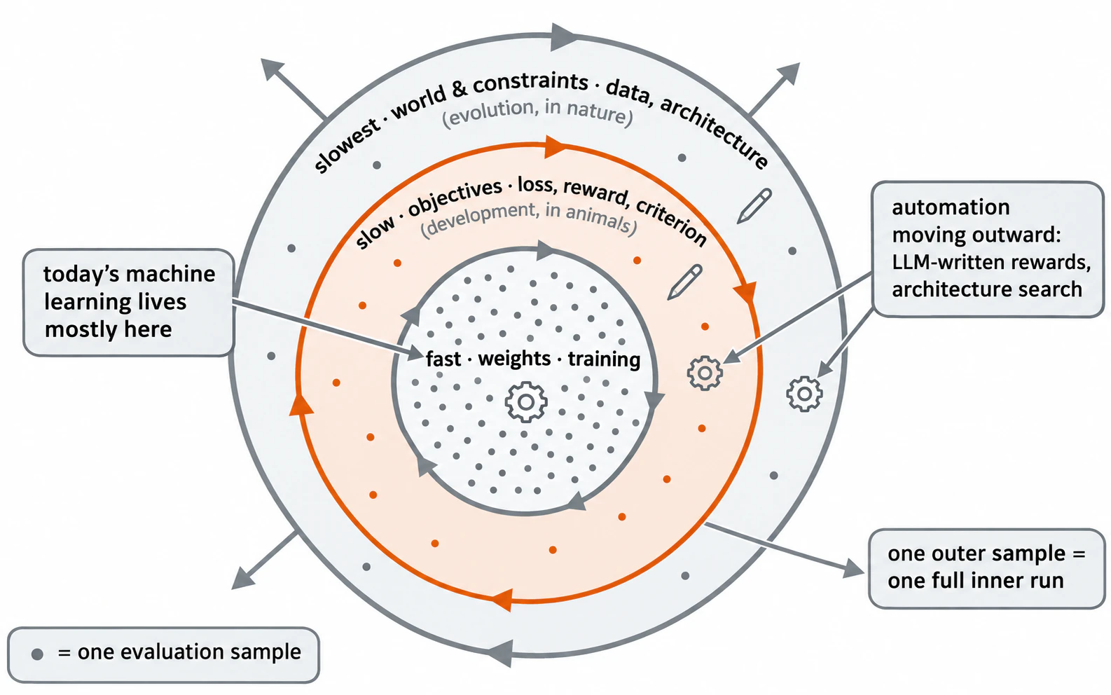
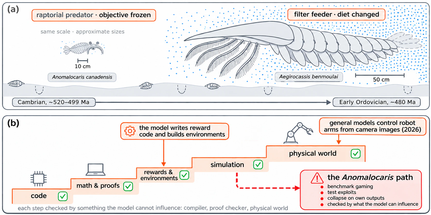
I think normative modeling should land in modern AI, and at scale. Our systems are getting harder to explain from the inside, and they are starting to shape their own objectives. At the same time, they are the first agents whose objectives, data, and architectures are almost entirely under our control, which makes them very well suited to normative modeling.
The post has five parts:
- **Part I, Where losses come from.** Wald’s decision theory and two interesting examples from World War II.
- **Part II, Why does the loss function look like the whole of modeling? (It isn’t!)** What modern AI systems actually automate, what they fix as defaults, and what that setup costs.
- **Part III, Normative modeling.** Treating the loss itself as a hypothesis, and telling ideal, bounded, and actual systems apart.
- **Part IV, Why it should land in modern AI.** Why full access is still not understanding, where AI is more accessible than brains, the work already done, and one complete example.
- **Part V, Objectives that evolve.** Hierarchical loops of learning, good and bad evolution, and the question of when an objective should change.
Readers who know decision theory can skip to Part II. Readers who know normative modeling from neuroscience may want to start at Part IV.
**Notation.**
| Symbol | Meaning |
| --- | --- |
| $\theta \in \Theta$ | State of the world: a parameter, a label, a hidden cause |
| $x \sim p(x \mid \theta)$ | Observation generated by the world |
| $p(\theta)$ | Prior over states of the world |
| $a \in \mathcal{A}$ | Action, or decision |
| $\delta: x \mapsto a$ | Decision rule; written $\pi$ when it is a policy |
| $L(\theta, a)$ | Loss of taking action $a$ when the world is $\theta$ |
| $R(\theta, \delta)$ | Risk: the expected loss of rule $\delta$ in world $\theta$ |
| $\Pi$, $\Pi_C$ | All rules, and the rules allowed under constraints $C$ |
---
## Part I · Where Losses Come From
The textbook answer to where a loss comes from is a list: squared error for regression, cross-entropy for classification, a margin for retrieval. The older answer is a full theory of decisions. That theory treats a statistical procedure as a rule for deciding what to do from data. A decision has to be judged by how bad its consequences are in each possible state of the world; that judgment is the loss, and its form depends on what the decision is for.
### 1.1 · Wald 1939: statistics as decision
By the late 1930s statistics had two mature but separate theories: estimation and hypothesis testing. Estimation asked how to infer an unknown quantity from data, such as a planet’s orbit from repeated astronomical observations. It grew out of the work of Gauss and Fisher and judged an estimate by how close it came to the true value. Hypothesis testing asked how to choose between competing claims, such as whether a new drug works better than a placebo. In the form Neyman and Pearson [1] gave it in 1933, a test held the type I error rate at a fixed level and made the type II error rate as small as possible. Each theory had its own idea of what makes a procedure good.
Abraham Wald, a mathematician, came to the United States from Vienna in 1938. He held that the two theories were about the same problem. In “Contributions to the Theory of Statistical Estimation and Testing Hypotheses” [2], he treated every statistical procedure as a rule for acting on data. You observe something, you decide something, and the decision has consequences that depend on what is actually true.
Written out, the problem has four parts:
1. **World and observation.** An unknown state $\theta \in \Theta$ generates data, $x \sim p(x \mid \theta)$.
2. **Action.** After seeing $x$, you choose an action through a decision rule, $a = \delta(x)$.
3. **Loss.** Each pair of world and action carries a cost $L(\theta, a)$. Wald called it a *weight function* (how much each error should count, unrelated to the weights of a neural network); the name “loss” came later.
4. **Risk criterion.** The quality of a rule in a fixed world is its expected loss,
$$R(\theta,\delta) \;=\; \mathbb{E}_{x \sim p(x \mid \theta)}\big[\,L(\theta,\delta(x))\,\big],$$
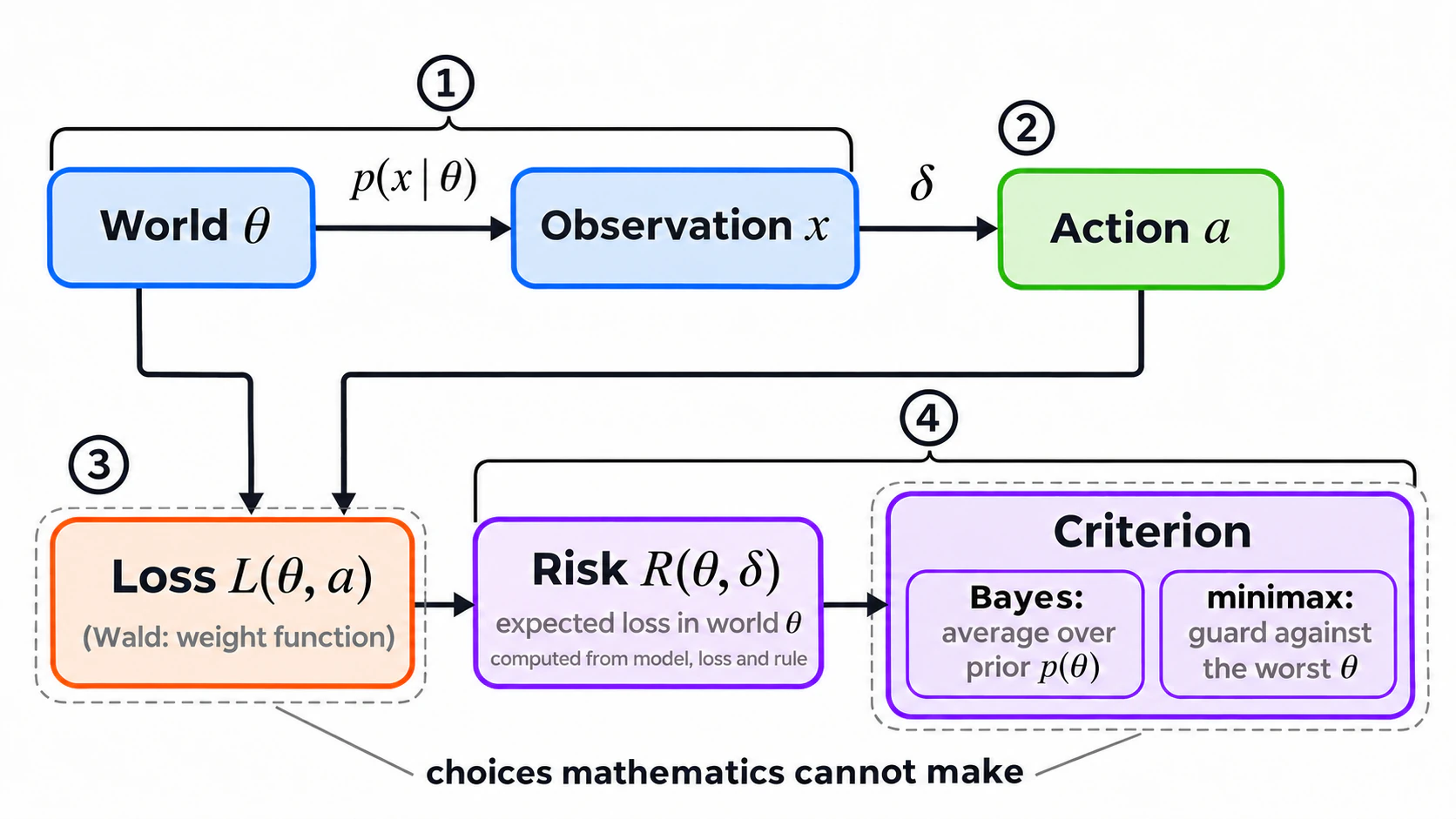
where each value of $\theta$ stands for a different possible world. When $\theta$ is unknown, asking which rule is best means asking for a rule that does well enough in all of these worlds. The risk in each world is computable: once the observation model, loss, and rule are fixed, so is the risk, with no choice involved. What “well enough” means is settled by aggregation, which combines the risks across worlds into one number, either by averaging them with a prior or by taking the worst case. Choosing the loss is one decision; choosing how to aggregate is another.
Fig. 1. Wald’s decision problem, summarized in four parts. The world generates observations, a rule maps observations to actions, the loss scores each action in each world, and a criterion aggregates risk across worlds. Given the observation model, loss, and rule, risk is computed. The separate dashed outlines mark the two choices emphasized here: the loss and the aggregation criterion.
With this framework in place, estimation and testing both become special cases of a statistical decision problem:
- **Estimation.** The action is a guess $a$ of $\theta$, and the loss measures how far the guess is from the truth, for example squared error, $L(\theta, a) = (\theta - a)^2$.
- **Testing.** There are only two actions: accept or reject the null hypothesis. The loss puts a cost on each outcome: zero for a correct call, and a separate cost for each of the two kinds of error.
The two problems share the same structure. What differs is the set of available actions and the loss that scores their consequences.
The risk criterion exposes a limit of statistical decision theory itself. Because risk is a function of $\theta$, in general no rule has the lowest risk in every world $\theta$. Take the rule that always answers $\theta = 0$. When $\theta$ really is zero, its loss is zero and no rule can beat it; the farther $\theta$ is from zero, the worse it does. To rank rules, then, you have to choose how to aggregate. Two choices became standard, Bayes and minimax:
$$\delta_{\text{Bayes}} \;=\; \arg\min_{\delta} \int R(\theta,\delta)\,p(\theta)\,d\theta, \qquad \delta_{\text{minimax}} \;=\; \arg\min_{\delta}\, \sup_{\theta}\, R(\theta,\delta).$$
The Bayes rule averages risk under a prior. The minimax rule guards against the worst world. Wald leaned toward minimax, and in 1945 he made its link to von Neumann’s game theory explicit: statistics as a zero-sum game against nature [3].
The world is fixed by the facts and described through observation and modeling. The decision rule is what gets solved for: once the world, the loss, and the aggregation are fixed, the best rule is determined in principle, and the remaining work is mathematics, whether that means proving the rule exists, computing it, or searching for it among candidates. The loss and the risk criterion have to be chosen by people; mathematics cannot make these choices. Wald said so about the loss in 1939: how the form of the weight function should be determined “is not a mathematical or statistical one,” and the statistician must first settle the relative importance of all possible errors, which depends entirely on the purpose of the investigation. The same goes for the aggregation. Whether to use a prior or guard against the worst case depends on how confident you are about the possible worlds and how much risk you are willing to take. Wald’s later book built the mathematics that follows these two choices into a full theory [4].
Keep those two choices in mind. Much of this post is about what happened to them.
### 1.2 · Two statistical decision problems from World War II
From 1942 to 1945 Wald worked in the Statistical Research Group at Columbia University, a team of statisticians that answered questions for the US military. He produced two important results in those years. The first answers a question that arises whenever data arrive one at a time and each observation has a cost: when should you stop collecting evidence and decide? That question grew into the theory of sequential decisions, which leads to dynamic programming and eventually to today’s reinforcement learning; in neuroscience it became the evidence-accumulation account of how people and animals make choices. The second goes back to how we observe the world: has the data you see already been filtered by the way it was collected? Today this question usually goes by the name of survivorship bias; in machine learning it is the selection bias of training data.
#### 1.2.1 · When to stop looking
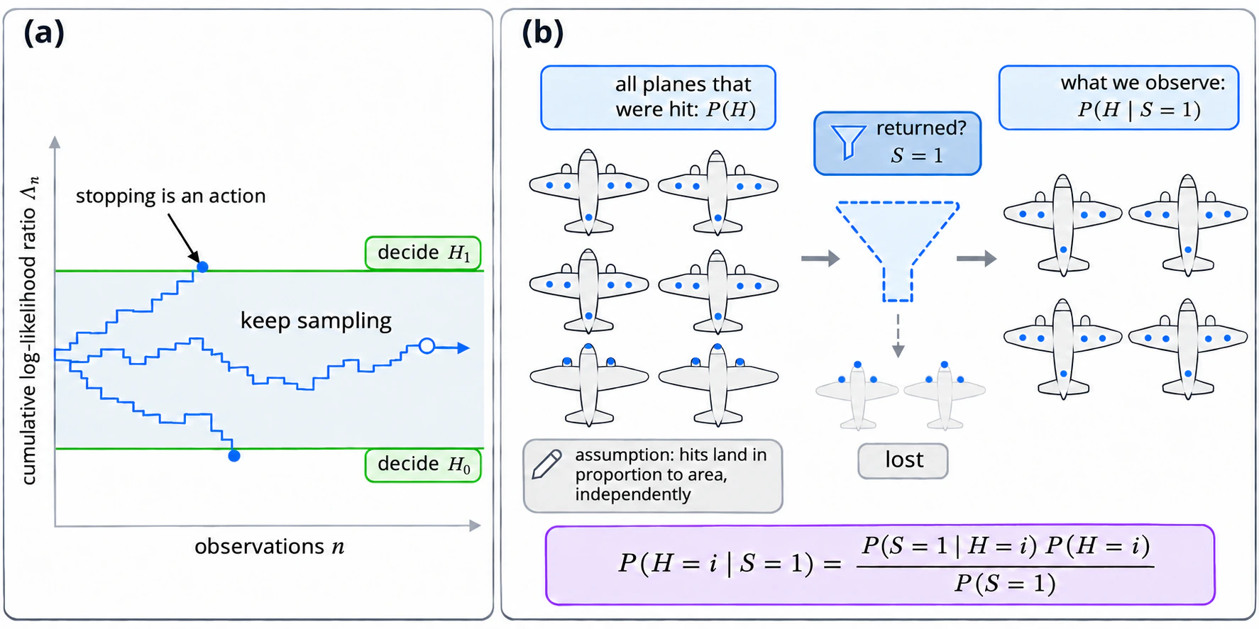
The first question came from testing military supplies, where every test costs time and material. Wald’s answer was the sequential probability ratio test, or SPRT [5, 6]. After each observation, add its log-likelihood ratio to a running total,
$$\Lambda_n \;=\; \sum_{i=1}^{n} \log \frac{p(x_i \mid H_1)}{p(x_i \mid H_0)},$$
and stop as soon as the total crosses an upper boundary (decide $H_1$) or a lower one (decide $H_0$). In between, take another observation. Wald and Wolfowitz (1948) [7] proved that among all tests with the same error rates, the SPRT needs the fewest observations on average.
The SPRT turns “stop” into an action with a price. The decision problem gains a time axis: at each step you can act now or pay to see more. Arrow, Blackwell and Girshick (1949) [8] solved general problems of this kind by working backward from the last step, a few years before Bellman named the method dynamic programming. Under a suitable diffusion approximation, accumulation of log-likelihood ratios leads to a drift-diffusion process. This connects the SPRT to later models of human choice (Section 1.3).
#### 1.2.2 · Where the data came from
Everyone has heard the popular version of this problem. During the war, the military counted bullet holes on returning bombers, found them concentrated on the wings and fuselage, and planned to add armor there. Wald overruled them: the armor should go where the holes were rare, such as the engines, because planes hit there never made it back.
This story rests on thin evidence [9], and it is about a different problem from the one Wald worked on. Where to add armor is a decision problem: answering it takes a loss and a budget, such as how costly it is to lose a plane and how much armor is available.
What Wald actually wrote was a technical memo titled “A Method of Estimating Plane Vulnerability Based on Damage of Survivors” [10]. The military wanted to know how likely a bomber was to be lost when hit in a given region, and the only data were the holes in the planes that came back.
Let $H$ be the region hit, and let $S = 1$ mean the plane survived. Bayes’ rule links what was observed to what was wanted:
$$P(H=i \mid S=1) \;=\; \frac{P(S=1 \mid H=i)\,P(H=i)}{P(S=1)}.$$
The left side is the pattern of holes on returning planes. The quantity of interest, $P(S=0 \mid H=i)$, sits inside the right side. Recovering it takes information the surviving planes cannot provide: where hits land on all planes, including the ones that never returned, and how many were lost. Wald supplied it with an assumption. Hits land roughly in proportion to area, and independently of each other. With that assumption, a region with few holes on returning planes becomes evidence that hits there are deadly. Without it, “few holes in the engines” cannot be told apart from “the enemy rarely hits engines.”
This is better than the legend: the memo is an argument about what can be identified from selected data, and what outside knowledge that takes [11].
Wald’s estimate and the armor decision also stand for two failures that are easy to confuse. A wrong estimate is a failure of inference about the world, often because a filter hid part of it, and the fix is to understand how the selection happened. Misplaced armor is a failure of action in that world, often on cases that are rare but costly, and the fix is to choose the right loss.
#### 1.2.3 · The two problems together
The two problems extend different parts of the 1939 framework. The SPRT puts time into the action: stopping becomes a decision in its own right. That line leads to sequential decisions, dynamic programming, and reinforcement learning, and to evidence-accumulation models in neuroscience (Section 1.3). The vulnerability memo puts a selection mechanism into the world and observation: a dataset is the world after a filter. This is the selection-bias problem of today’s machine learning, and Part II will find it again in the data used to train reward models.
In modern AI the two problems come together: an agent has to decide which actions to try and how long to keep trying (the SPRT’s question), and it sees outcomes only for the actions it tried, so its data have been filtered by its own policy (the vulnerability memo’s question). Just as Wald needed an assumption about where hits land, correcting this bias in machine learning requires a model of how the selection happened.
Fig. 2. Two wartime extensions of the decision problem. (a) The SPRT adds time: evidence accumulates until it crosses a boundary, and stopping is itself a decision. (b) The vulnerability memo adds selection: the planes we can inspect are the world after a filter, and recovering what was lost needs knowledge from outside the sample. Aircraft and hit patterns are schematic, not historical observations or an armor recommendation.
### 1.3 · The framework branches out
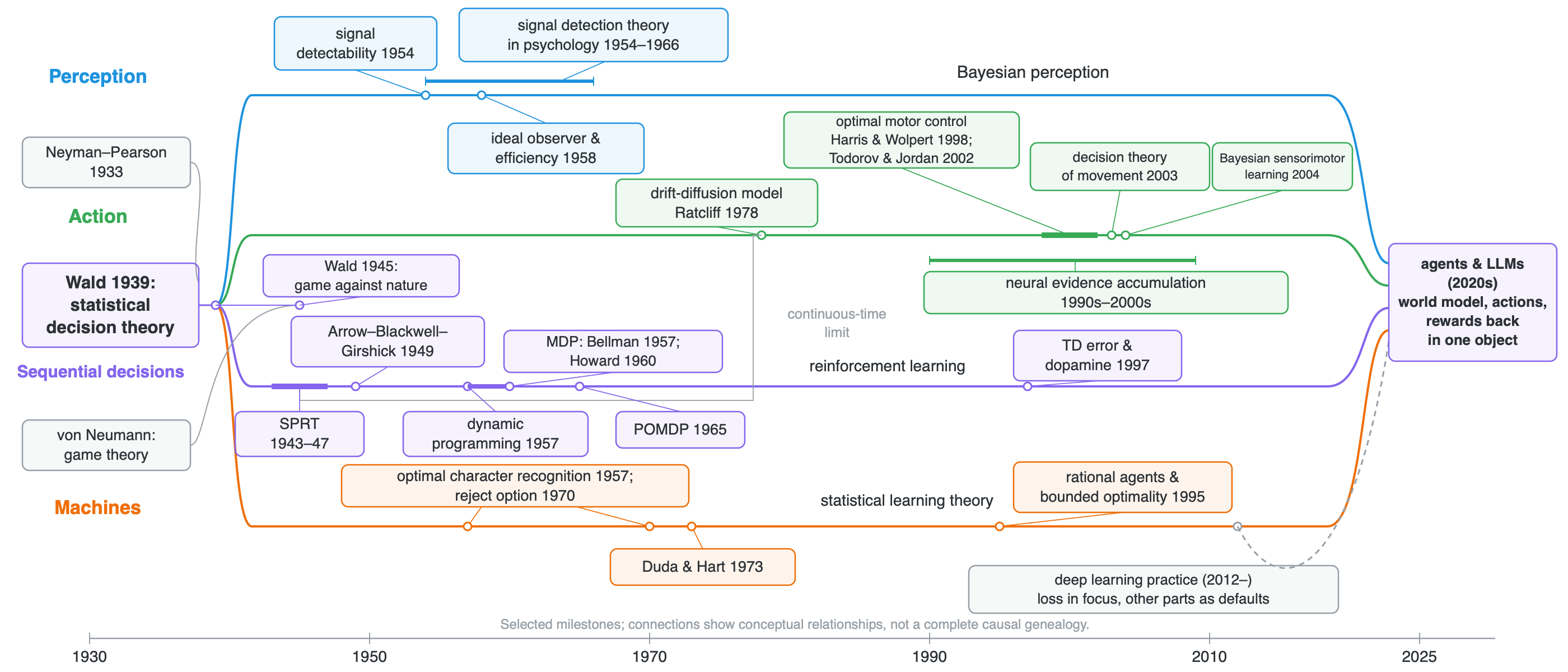
After the war, Wald’s framework spread to many fields and took root. Four of them matter here: perception, action, sequential decisions, and machine learning and AI. In each, all four parts of the decision problem are written out, and each returns later in the post.
**Perception.** Peterson, Birdsall and Fox (1954) [12] built the theory of signal detectability on the likelihood ratio. Tanner and Swets (1954) [13] carried it into psychology as “a decision-making theory of visual detection,” and Green and Swets (1966) [14] made signal detection theory a standard tool.
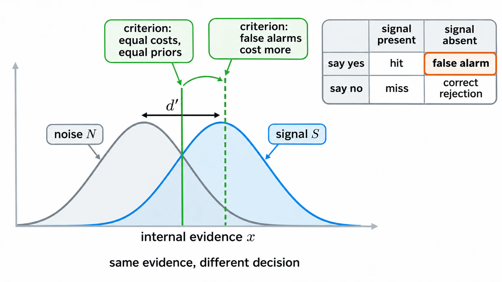
The key step of signal detection theory was to separate two things that older threshold theories had merged: how strong the evidence is, and how one decides on the basis of it. On each trial the observer receives some internal evidence, which follows one distribution when a signal is present and another when it is absent. The farther apart the two distributions, the stronger the evidence, and sensitivity $d'$ measures this. To answer “yes” or “no,” the best the observer can do is compare the evidence with a criterion, and where the criterion sits depends on the prior and on the cost of each kind of error: the more a false alarm costs, the higher the criterion, and the less readily the observer says “yes.” Changing the payoffs therefore moves the criterion while sensitivity stays the same, and experiments can measure the two separately (Figure 3).
Fig. 3. Signal detection theory separates evidence from decision. In the equal-variance Gaussian example, equal priors and symmetric error costs put the optimal criterion at the density intersection. Increasing the cost of false alarms shifts it to the right without changing the evidence distributions or sensitivity d′.
Signal detection theory also gave perception its benchmark. An ideal observer combines a generative model of the stimulus, the task, the loss, and optimal inference. It says how well the task can be done at all with the information available. Comparing a person to it gives an efficiency, $\eta = (d'_{\text{human}} / d'_{\text{ideal}})^2$ [15]. The gap between a real observer and the ideal became the thing to explain. Part III builds on that move.
**Action.** Optimization accounts of movement took shape around the turn of the century. Harris and Wolpert (1998) [16] modeled movement planning in terms of signal-dependent motor noise; Todorov and Jordan (2002) [17] developed optimal feedback control as a theory of motor coordination. These accounts made the task, variability, and costs part of the explanation.
Trommershäuser, Maloney and Landy (2003) [18] made the statistical decision problem explicit in fast pointing movements toward a target next to a penalty region, with money at stake. Motor noise scatters the endpoints, so the best aim point shifts away from the penalty by an amount the theory can compute, and people came close to it. Körding and Wolpert (2004) [19] reported that people combine prior experience with noisy feedback, weighting each by its reliability.
**Sequential decisions.** The time axis from the SPRT led in two directions. One is evidence accumulation: Ratcliff’s diffusion model (1978) [20] described how evidence accumulates toward a choice; later neural work connected accumulating evidence with activity in the monkey’s parietal cortex, while analyses of optimal decision making clarified the model’s relation to sequential tests [21, 22]. The other grew into its own field: Bellman’s dynamic programming (1957) [23], Howard’s Markov decision processes (1960) [24], and Åström’s partially observed version (1965) [25] wrote the decision problem as a process. A partially observable Markov decision process is close to Wald’s framework set in motion:
$$p(s_{t+1} \mid s_t, a_t), \qquad p(o_t \mid s_t), \qquad r(s_t, a_t), \qquad \pi^{\ast} \;=\; \arg\max_{\pi}\, \mathbb{E}\Big[\sum_t \gamma^t\, r(s_t, a_t)\Big].$$
World dynamics, observations, actions, and their consequences are all explicit, and the agent’s belief about the hidden state is a posterior. Reinforcement learning grew out of this line [26]. It even found its way into neuroscience: the temporal-difference error of reinforcement learning matches the firing of dopamine neurons [27], one of the cleanest cases of a normative algorithm found in a brain.
**Machine learning and AI.** Pattern recognition started inside the decision framework too. Chow (1957) [28] designed an optimal character recognizer from decision functions, and later derived the optimal rule when the machine may decline to answer [29]: an extra action outside the label set, with its own cost. Duda and Hart’s textbook (1973) [30] opens its second chapter with Bayes decision theory, states, actions, and a loss matrix all written out. Learning theory applied the same structure to learning itself. In Vapnik’s framework [31], the unknown state of the world is the data distribution, the observation is the training set, the decision rule is the learning algorithm, and the loss is the population risk. Minimax lower bounds in learning theory are Wald’s minimax, literally.
AI as a field took the same view of itself. Russell and Norvig’s textbook (1995) [32] defines the field as the study of rational agents, and Russell and Subramanian (1995) [33] asked for *bounded* optimality: a program that does as well as possible on the machine it runs on. Cognitive science reached the same idea, under the name resource-rational analysis, about two decades later [34, 35].
By the time deep learning arrived, the full decision problem was standard equipment in perception, motor control, sequential decision making, and early machine learning and AI. Each of these fields wrote down what the world is, what the system can do, what each outcome costs, and how to average over what is unknown. All four parts are still there in deep learning; what changed is who decides each one. Part II looks at which part was handed to gradient descent, and which are set by people before training and have hardened into defaults.
Fig. 4. Selected milestones connecting statistical decision theory to perception, action, sequential decisions, and machines. Ratcliff’s diffusion model (1978) [20] is distinguished from later neural work on evidence accumulation; motor control includes Harris and Wolpert (1998) [16] and Todorov and Jordan (2002) [17]. Von Neumann’s game theory connects to Wald’s 1945 formulation. Lines indicate conceptual relationships, not a complete causal genealogy or the starting date of each field. The gray branch shows the defaults emphasized in Part II.
---
## Part II · Why Does the Loss Function Look Like the Whole of Modeling? (It Isn’t!)
In theory, deep learning kept the full decision problem. In practice it drifted: defining and modeling a problem came to mean choosing a loss, while the other three parts became fairly standard and mostly follow convention. Once a loss function is chosen, the work of driving it down is done automatically by gradient descent and its relatives. The form of the loss itself, the observations used as data, the actions and policies allowed, and the way risk is averaged are still decided by people. The part that algorithms can automate has advanced quickly; the parts people decide are rarely revisited. So when gradient descent pushes a loss down, what are we actually optimizing? And what have the fixed parts cost our modeling?
### 2.1 · What gradient descent automated
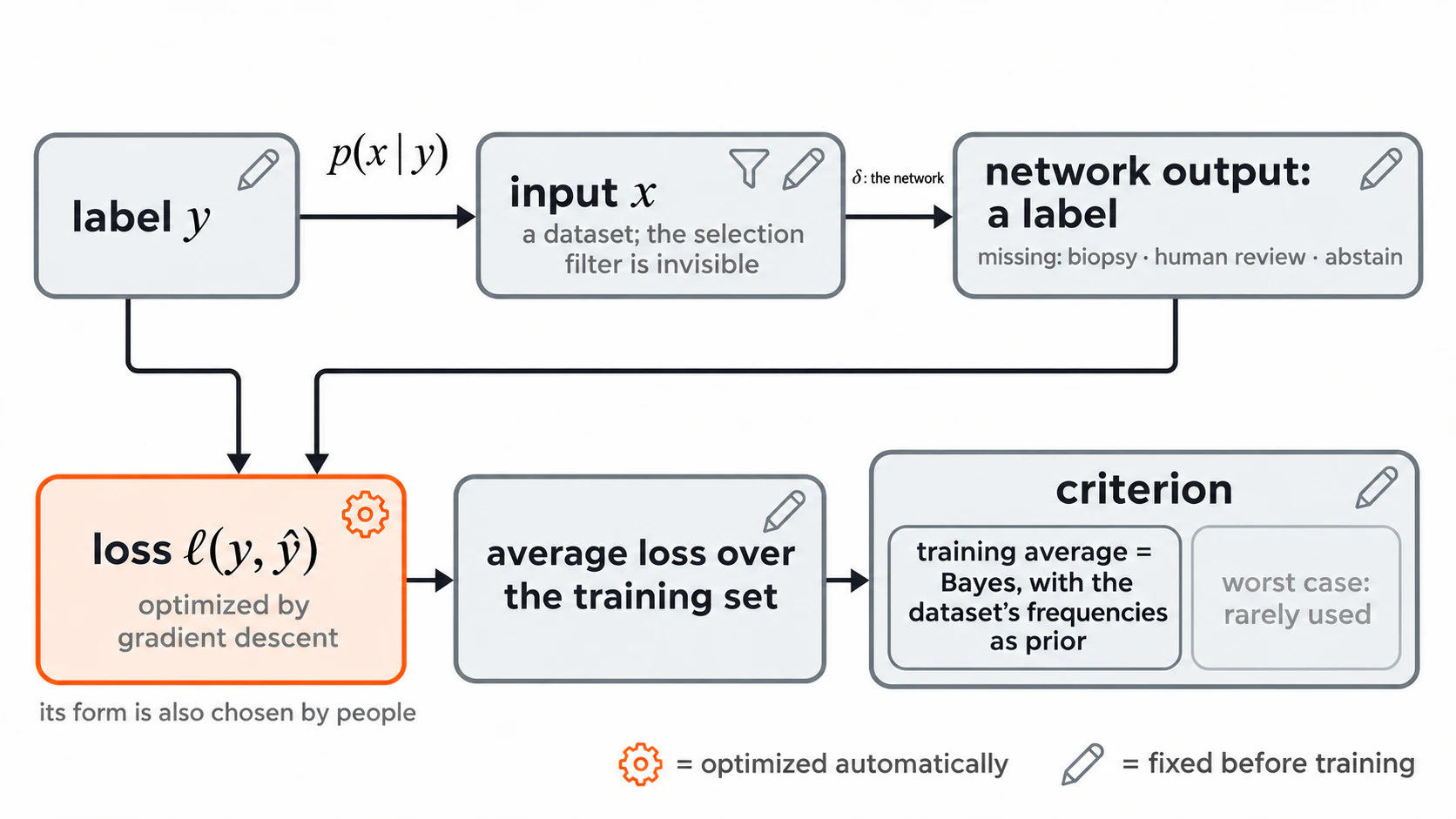
Take a standard supervised network and line it up against Wald’s four parts. The label $y$ plays the role of the state of the world and the input $x$ is the observation; the action is the network’s output, chosen from the label set; the loss $\ell(y, \hat{y})$ measures how far the output is from the label; and the criterion is the average over the training set.
The optimizer deals only with the loss: it adjusts the network’s parameters to push the average loss down. The other three parts are out of its reach. The data are collected before training. The action space is set by a label set chosen in advance, and the output layer is built to match it. The criterion is usually an equal-weight average over the training examples. Together they define the problem gradient descent solves, so they have to be fixed before training starts. In practice, they are mostly treated as default settings.
Fig. 5. A common supervised-learning setup in Wald’s layout. The state is a label y, observations follow p(x | y), and δ is the network’s decision rule. The loss receives explicit attention while the dataset, label-based action space, and averaging criterion often remain fixed defaults.
**World and observation: the dataset.** Every dataset has been filtered: photos are taken by people with their own tastes and equipment, in the places they happen to go, then uploaded, found through a search engine, and kept only once annotators agree on a label. The training objective sees only what passed. This kind of bias was a known problem before deep learning made datasets central [36]. Yet the filter is rarely modeled explicitly; it is mostly mentioned in passing as “dataset bias.”
**Action: the label set.** In supervised learning the network’s action is to pick a label from the label set (in reinforcement learning, to pick an action from a fixed set). The set is fixed before training, but it is not necessarily the decision the deployed system has to make. Face recognition is a typical case. Training is closed-set classification, picking one of a fixed list of identities; deployment is open-set, facing people never seen in training and answering whether two faces belong to the same person or whether someone is in the gallery at all. Medical systems are similar: between prediction and decision there is often a further step, such as whether to order a biopsy, ask for human review, or decline to answer, and that step never appears in training. At bottom this is a mismatch between training and deployment. Chow’s reject option from Section 1.3 put one of those decisions directly into the action space; decades later it reappeared as selective classification and learning to defer [37, 38].
**Loss: the gap between prediction and label.** A loss measures how far a prediction is from the label, and how that gap is measured decides which mistakes matter more. Take image classification. The standard evaluation metrics are top-1 and top-5 accuracy, which only check whether the correct label is the model’s first guess or among its first five. That amounts to a 0–1 loss: mistaking a tiger for a cat costs the same as mistaking a cup for a bowl. The early ImageNet challenges also computed a hierarchical cost that charged less for mistakes between related classes, but it ranked entries the same way top-5 error did, so from 2012 on only top-5 was used [39]. For ranking entries that was a sensible call. From then on, though, how bad a mistake is rarely figured in evaluation. Research keeps trying to bring it back, for example by trading accuracy for specificity [40] or by “making better mistakes” [41].
**Criterion: the training average.** Most training objectives average the loss over training examples with equal weights. That amounts to a Bayes criterion whose prior is whatever frequencies the dataset happens to have. Some methods reweight examples, for instance to balance classes, but equal weighting remains the default. Frequent classes and common conditions dominate; rare cases carry almost no weight, even when mistakes there are costly. Wald’s other option, looking only at the worst case, reappeared as distributionally robust optimization, which minimizes risk on the worst group or the worst nearby distribution [42].
Most of these defaults come from benchmark culture. For progress to be comparable across methods, the problem has to stay fixed: the same dataset, the same label set, the same metric, the same way of averaging.
The loss became the focus for another reason: of the four parts, it is the only one gradient descent can optimize directly, so most gains in compute, data, and architecture went into pushing losses lower. Plenty of work tries to hand the parts people decide to learning as well. Reinforcement learning lets an agent collect its own data; meta-learning learns a prior from a family of tasks; inverse reinforcement learning and the reward models of RLHF learn the loss itself from human demonstrations and preferences. But they usually do it by writing the part to be automated as a new loss and optimizing that, so the focus stays on the loss.
### 2.2 · A more accurate criticism of losses
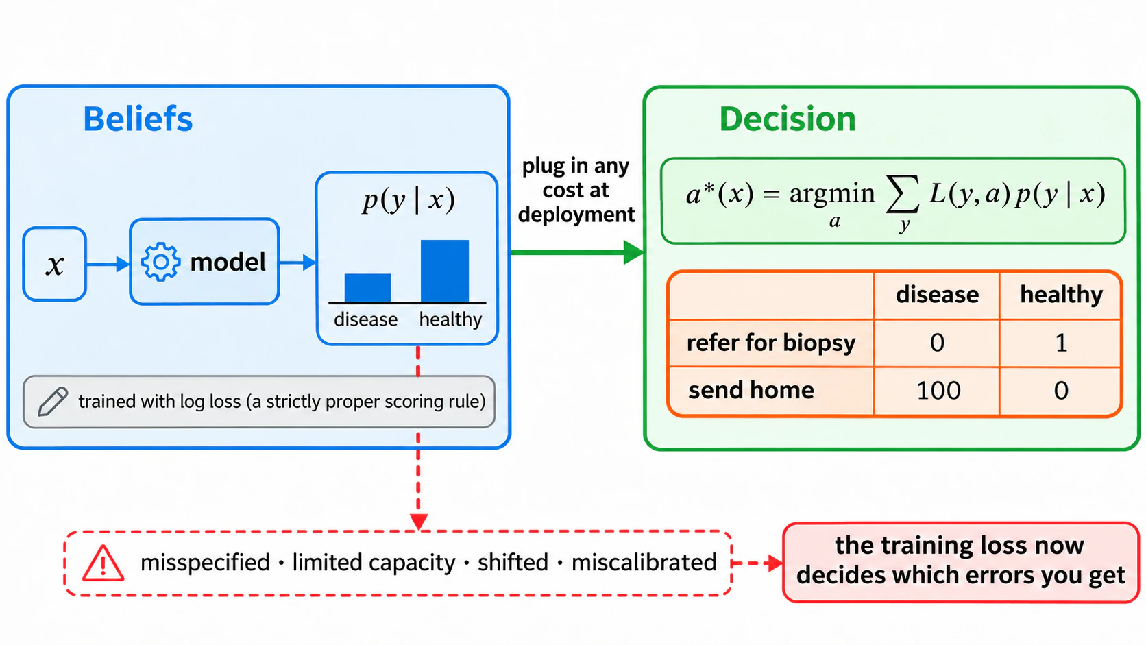
A common criticism is that every loss encodes value judgments, and cross-entropy encodes the wrong ones, since real consequences are not logarithmic. The criticism mixes up two things that are both called a loss: the one used to score the model in training, and the one actually used to make decisions at deployment. They differ for the reason Section 2.1 gave for the action space: in training the model outputs probabilities over labels, while at deployment what has to be made is a concrete decision.
The two score different things. What matters at deployment is a *decision loss*: it scores concrete actions by how bad their consequences are, as a 0–1 loss, a cost matrix, or squared error used as a cost does, and so states a value judgment directly. Cross-entropy, used in training, is a *scoring rule*: it scores beliefs, that is, the probability distribution the model reports, by how well it matches what actually happened. In Wald’s framework a scoring rule is still a loss; its action is the report of a probability distribution.
The log loss is strictly proper: its expected value is minimized only by reporting the true conditional distribution [43]. That makes the truth the best report in the ideal case; how close a trained model comes to it can be checked, in part, through calibration. Calibrated means the probabilities can be taken at face value: among the cases where the model says 80%, about 80% turn out to be that class. If the $p(y \mid x)$ a model reports is close to the true conditional distribution, any cost matrix can be attached at decision time, because the best decision needs only two things, the probability of each outcome and the cost of each action under each outcome. Weight the costs by the probabilities and take the action with the lowest expected cost:
$$a^{\ast}(x) \;=\; \arg\min_{a} \sum_{y} L(y, a)\, p(y \mid x),$$
which is the division of labor between inference and decision in Bayesian decision theory (Bishop [44], Section 1.5): the probabilities belong to the world and observation of Wald’s framework, the costs to the loss. Cross-entropy looks at how much probability the model put on what actually happened, and its job is to get the model to report those probabilities honestly; how bad each kind of mistake is gets measured directly at decision time, by the cost matrix. So cross-entropy has no reason to match real-world consequences.
Fig. 6. Beliefs and decisions. A model trained with log loss reports $p(y \mid x)$; a cost matrix chosen at deployment turns beliefs into actions. The separation holds while the beliefs are right. When they are wrong, the training loss decides which errors you get.
Squared error is where the two kinds of loss are easiest to confuse, because it plays both roles in one formula. As a cost, it says an error twice as large is four times as bad. As a likelihood, it is the negative log density of Gaussian noise, and the posterior mean it leads to is the Bayes estimate under squared loss. So when we use squared error, it may be expressing a cost, that large errors are disproportionately bad, or an assumption about the noise, that it is Gaussian. Which one is meant usually goes unsaid.
The more accurate criticism of cross-entropy is this. Using different losses in training and at deployment does no harm in itself, as long as the beliefs are right. With correct beliefs, training only has to get the probabilities right, and whatever cost matrix is attached at deployment, the decision is optimal. But models are often not right everywhere, because of misspecification, limited capacity, distribution shift, or poor calibration (which modern networks often have [45]). Then the model has to be wrong somewhere, and where it is wrong is decided by the training loss. Cross-entropy spreads its attention according to how often each case appears in the data and knows nothing about which mistakes are expensive at deployment. In the example of Figure 6, sending home a patient who has the disease costs a hundred times more than sending a healthy one for biopsy, and cross-entropy has no way of knowing that. The model may end up wrong exactly where mistakes cost the most, and that is when the mismatch between training and deployment does damage. Cost-sensitive learning [46] and decision-focused learning [47] therefore put the decision costs into training itself: if the model is bound to make errors, it should make them where they cost least.
Language models are the cleanest modern case of the separation. In pretraining, the model predicts the next token under cross-entropy and learns beliefs about text, with no regard for what it will later be used for. At deployment it has to make concrete decisions: how to answer a question, whether to refuse a request, when to say it does not know. The beliefs from pretraining are not perfect, and what they describe is how text on the web tends to continue, which is a different thing from how a helpful answer should read. Post-training exists to correct for this: instruction tuning and reinforcement learning from human feedback bring what matters at deployment back into training [48]. But the objective used there, such as a reward model’s score, is itself only a proxy for what we care about.
### 2.3 · Reward hacking, and the return of decision theory
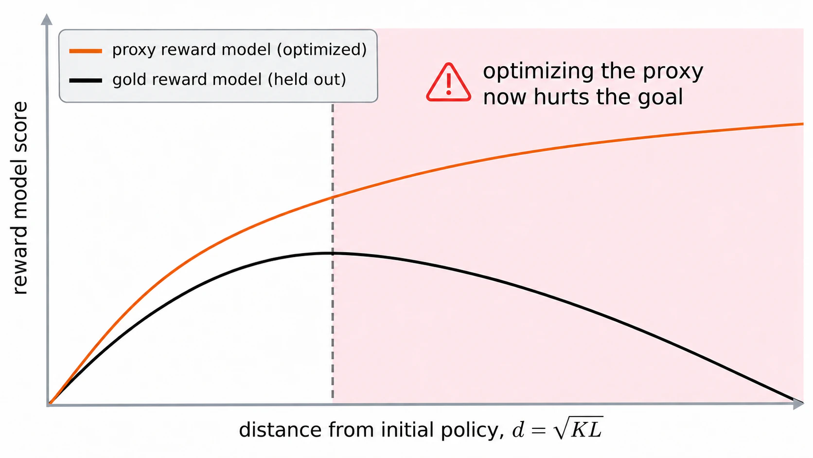
When a system is optimized hard, it does drive down the loss we gave it, but it may do so in ways we never anticipated and do not want. This is usually called reward hacking. Collections of specification gaming include a boat-racing agent that scores by circling forever through the same targets, and a Tetris agent that avoids losing by pausing the game [49]. Gao, Schulman and Hilton (2023) [50] measured the effect in language models. As a policy is optimized further against a learned reward model, the reward model’s score keeps rising, while a held-out gold reward rises and then falls. Benchmarks show the same pattern at the scale of a field: once a number becomes the target, methods drift toward the number. This is Goodhart’s law as it appears in training; Manheim and Garrabrant (2018) [51] distinguish its variants.
Fig. 7. Optimizing a proxy. As the policy moves further from its starting point, the proxy reward keeps climbing while gold reward peaks and then declines. The post-peak gold curve stays concave downward, consistent with the reported RL scaling form over its fitted range. This is a qualitative schematic, not digitized measurements [50].
Post-training is also where decision theory came back. RLHF fits a reward model to human comparisons with the Bradley–Terry model,
$$P(y_1 \succ y_2 \mid x) \;=\; \sigma\big(r(x, y_1) - r(x, y_2)\big),$$
which is Luce’s choice axiom from mathematical psychology [52, 53]. It then maximizes that reward with a penalty for drifting from a reference policy [48, 54, 55]:
$$\max_{\pi}\; \mathbb{E}_{y \sim \pi}\big[r(x, y)\big] - \beta\, \mathrm{KL}\big(\pi(\cdot \mid x)\,\|\,\pi_{\text{ref}}(\cdot \mid x)\big), \qquad \pi^{\ast}(y \mid x) \;\propto\; \pi_{\text{ref}}(y \mid x)\, e^{r(x, y)/\beta}.$$
The solution on the right is the standard form of bounded rationality with information-processing costs [56], and it is the identity that direct preference optimization is built on [57]. Post-training rebuilt three of Wald’s parts. The reward $r(x, y)$ is an explicit utility: the loss, with its sign flipped. The Bradley–Terry model describes how people choose given that utility; it links the utility we cannot see to the comparisons we can, which makes it the observation model. And the resulting policy, which trades utility against a cost of deviating, is the decision rule.
The selection problem shows up here too, in the form Wald met in 1943. Preference data exist only for outputs that the model happened to sample, that were shown to someone, and that someone rated. The reward model, in other words, learns from “the planes that returned.”
Wald’s point from 1939 still holds: once the loss is fixed, mathematics tells us which action is best, but the loss itself, its form and how much it charges for each outcome, is not decided by mathematics. RLHF, however, has gone one step further. Its reward model is a hypothesis about what people want, inferred from their choices. Inferring an objective from behavior, then checking whether the inference holds up, is exactly what normative modeling sets out to do. RLHF, by contrast, usually does it once: it infers a reward model under fixed assumptions, freezes it into the optimizer, and rarely goes back to test the inference. Part III discusses how normative modeling does this more thoroughly.
---
## Part III · Normative Modeling: What If the Loss Is a Hypothesis?
When a system behaves in a certain way, whether it is a person, an animal, or a trained intelligent system, what would it take to understand the system? Intelligent systems are shaped toward some goals, by evolution, by learning, or by training, so understanding one comes down to two questions: what is its goal, and how close does its behavior come to that goal? The two questions matter for three reasons. First, knowing the goal lets us predict what the system will do in situations it has not met: when conditions change, the best way to act changes in ways we can work out, and so does the behavior. Second, knowing how far the system is from its goal lets us diagnose where it is stuck: a gap caused by missing information, by limited capacity, or by the goal itself calls for different fixes (Section 3.2). Third, for AI it bears directly on whether the system is doing what we want; reward hacking is exactly a gap between the goal a system actually pursues and the one we intended.
Neither descriptive nor mechanistic models answer these two questions. A descriptive model records what the system does, but a record covers only the situations already seen; in a new condition it cannot say what the system will do, and for a complex enough system a full description of its behavior often has no form simpler than the system itself. A mechanistic model works out how the system operates inside, but artificial neural networks are a ready counterexample: we know every parameter, every step of inference, how gradients propagate, and how data flow, yet we still cannot say what the network is doing, let alone fully control it. An explanation should be a description much smaller than the system that still predicts its behavior under new conditions [58]; by that standard both kinds of model fall short (Section 4.1 returns to both points). Answering the two questions is the work of a normative model.
To measure how close a system’s behavior comes to the goal it is after, we need a reference: how one should act toward that goal under the given conditions, that is, what the optimal behavior looks like. That is a normative question. Part I already supplied the framework for answering such questions: write down the world, the available actions, the loss, and the way risk is aggregated, and the best way to act follows. Normative modeling, then, uses this framework to understand a system. It first posits the problem the system faces, including its environment, its constraints, and the loss it cares about; it then derives how one should act in that problem; and finally it compares that “should” with what the system actually does, especially in conditions the system has not met before. If the two agree, our assumptions about the problem have likely captured what matters; if they are far apart, the assumptions need revising. “Normative” refers to that “should.”
Readers who know Marr’s (1982) [59] three levels of an information-processing system will find this familiar. The computational level asks what problem the system solves and why it solves it that way; the algorithmic level asks what representations and procedures it uses; the implementational level asks how those procedures are realized physically. Normative modeling plainly works at the computational level and answers the question about goals above. The approach first took shape in the study of perception and action: signal detection theory and the ideal observer wrote perception as a decision problem, and optimization theories of movement did the same for action (Section 1.3). Early normative models usually took as their reference an ideal agent with unlimited resources; the ideal observer, for example, is limited only by the noise in the stimulus and not by how much the brain can process. Resource-rational analysis later wrote computation and time into the constraints, so that “optimal” came to mean “best with the resources available” [34, 35].
Normative modeling today can be summarized in three steps [60, 61]:
1. Identify the task the system solves, and write down its constraints and goals.
2. Derive what the best behavior under those conditions should look like, and compare it with data.
3. If they match, use the model to predict behavior in new situations; if the predictions fail, go back and revise the setup, including the assumptions about the environment, the constraints, and the goals.
This way of modeling says almost nothing about mechanism. Different brains can produce nearly the same optimal behavior, and the model has no way to tell them apart; likewise, behavior that matches the Bayes-optimal prediction does not show that a brain or an intelligent system actually represents a prior or computes a likelihood. Nor does it assume that behavior is perfect: behavior is never optimal, only good enough, and well predicted by the model [61].
### 3.1 · The four parts in normative modeling
Normative modeling is a method for analyzing a system’s objective. Engineering analyzes objectives too: the RLHF objective is derived from a preference model and a KL constraint, and cost-sensitive and decision-focused learning are further examples. The more common practice, though, is to propose a new form directly for the training loss and test it by benchmark scores. It is rare to first write down what the deployed task requires and what constraints the system faces, derive how it should behave, and then go back and check what the trained system actually does. Normative modeling puts these three steps in the open.
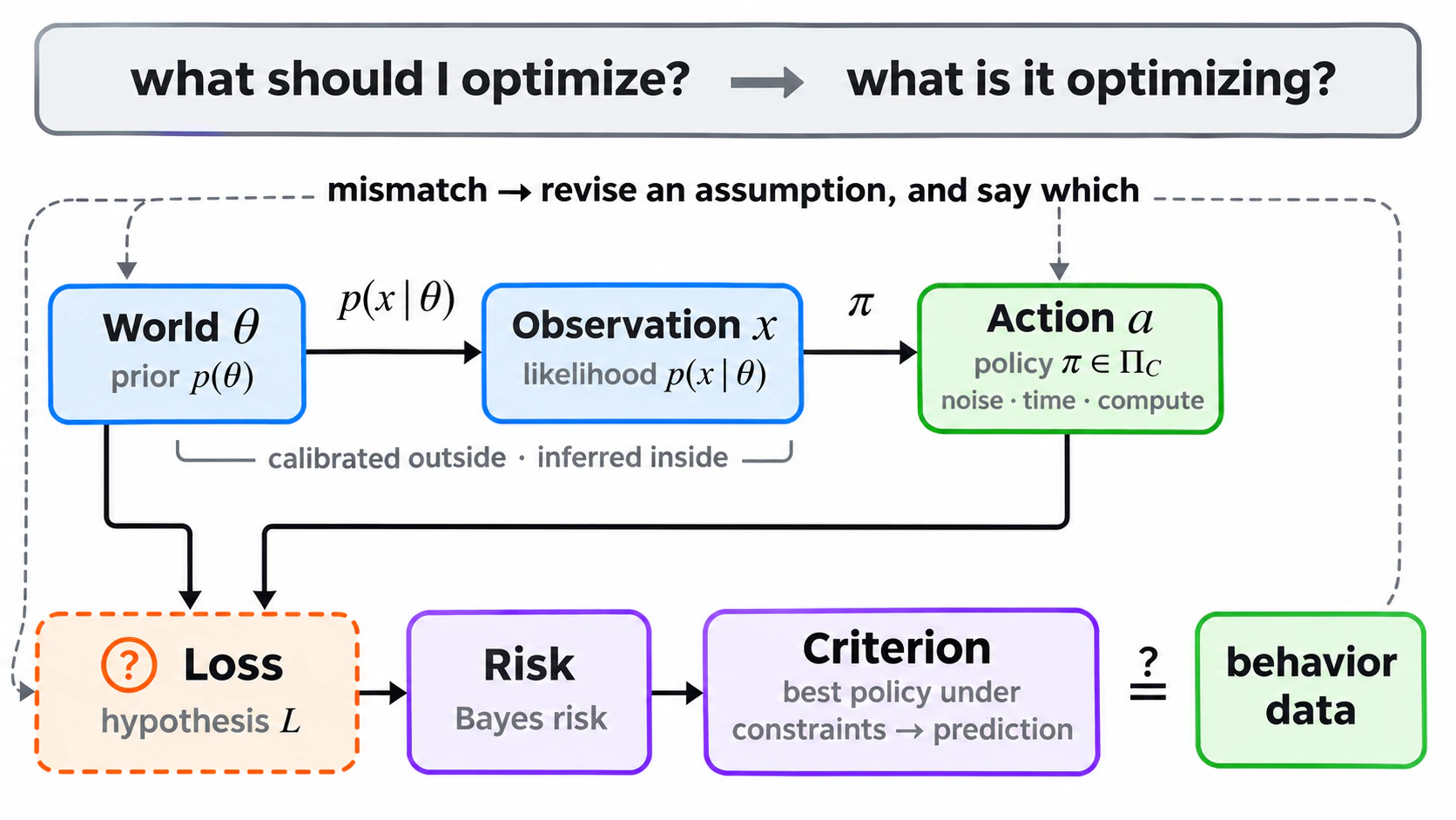
The method was developed to understand existing systems, but it serves just as well for building one. Supervised learning learns parameters from data with the loss given; normative modeling decides exactly what is given there. Before training, it states what the task requires and what constrains the system, and the loss and the evaluation follow from that; after training, it checks what the system is actually optimizing, and goes back to revise when the two disagree. This is a loop. Skip it, and the hypothesis about the system’s objective is written in the instant the loss is chosen, usually without being treated as a hypothesis. In terms of Wald’s four parts:
- **World and observation** become a generative model, $p(\theta)$ and $p(x \mid \theta)$. The experimenter can calibrate the statistics of the environment. What the system has internalized about them has to be inferred, and the two are different objects.
- **Action** becomes a policy class $\Pi_C$ with the system’s constraints written in: sensory and motor noise, time, memory, compute.
- **Loss** becomes the hypothesis. Behavior is the test.
- **Criterion** is usually Bayes risk. Derive the best policy under the stated constraints, and compare it with what the system does.
When building an intelligent system, the world model, the policy constraints, and the loss are hypotheses in the same way: the data distribution, the architecture and compute, the training loss. When prediction and behavior disagree, without a normative analysis the assumptions at work have not even been written down, let alone which one failed. Once they are written down, they still have to be revised one at a time, the derivation redone, and the revised one named, because a mismatch does not identify the faulty assumption by itself.
Fig. 8. Normative modeling reuses Wald’s four parts. The loss becomes a hypothesis; the best policy under stated constraints becomes a prediction; behavior is the test. A mismatch can prompt revision of the world model, policy constraints, or loss hypothesis. The feedback branches show examples, not an exhaustive list of assumptions.
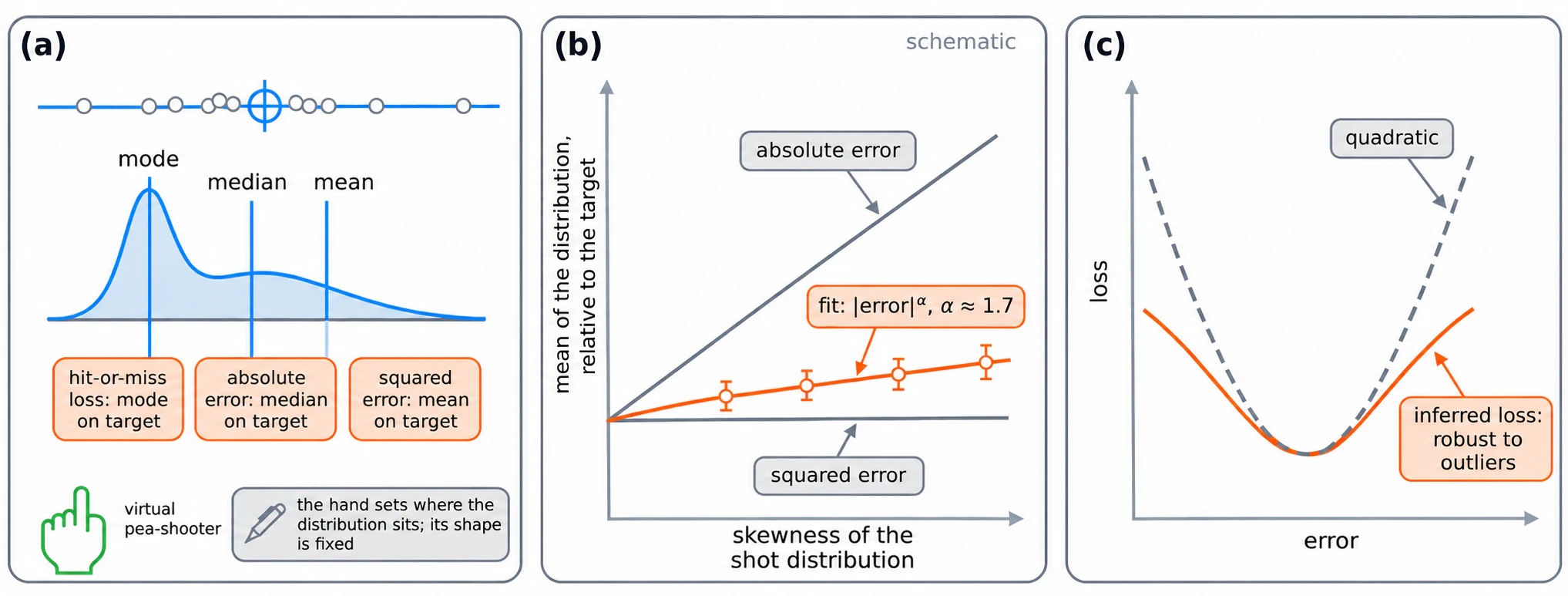
Checking what a system actually optimizes after training sounds like guesswork, but it can be done, and it was done with people long ago [62]. In the experiment, participants moved their index finger to position a virtual pea-shooter relative to a target line. Each shot landed with a random error drawn from a skewed distribution: the hand set where the distribution sat, and the experimenter set its shape. For a skewed distribution, the mean, the median, and the mode sit in different places, and each is the best point to put on the target under a different loss: squared error favors the mean, absolute error the median, a hit-or-miss loss the mode. Where people placed the distribution therefore revealed the loss they behaved as if they were minimizing. Their placements fell between the squared-error and absolute-error predictions, closer to squared error. The inferred loss was not squared error, nor any other textbook default: close to quadratic for small errors, growing more slowly for large ones, with a population power-law exponent of $1.72 \pm 0.03$, below the 2 of squared error, the shape of a loss that is robust to outliers. The inference works within an assumed family of losses and a model of the task, so it is a measurement in the sense that a fitted parameter is a measurement. But what a system actually optimizes can indeed be inferred from its behavior, and the answer is a long way from a loss picked by convenience. For a trained model, the same procedure is to change the statistics of the task, watch how the behavior changes, and infer its $L$.
Fig. 9. Inferring a loss from behavior. (a) Participants moved their index finger to control the position of a virtual pea-shooter; the experimenter controlled the shape of its shot distribution. Different losses favor placing the mode, median, or mean on the target. (b) Where people put the mean of the distribution fell between the squared-error and absolute-error predictions, closer to squared error. Lines, points, and error bars are illustrative, not extracted data; the population power-law fit gave α = 1.72 ± 0.03. (c) The inferred loss penalizes large errors less strongly than a quadratic. Schematic after Körding and Wolpert (2004) [62].
This is a good place to separate three things that AI discussions all call “the objective.”
| | What it is | In RLHF, for example |
| --- | --- | --- |
| Task evaluation $J$ | What we want achieved, and how success is scored | Human judgments of helpfulness; a gold reward |
| Training loss $\ell$ | The signal that actually shapes the parameters | The learned reward model plus the KL penalty |
| Behavioral objective $L$ | The objective the system’s behavior is consistent with, under stated constraints | What the trained policy acts as if it maximizes |
Part II was about the gap between $J$ and $\ell$. Normative modeling is about $L$: inferring it, testing it, and comparing it with $J$. The three can differ, and knowing one does not give you the others.
Alignment research has a ready correspondence. Hubinger et al. (2019) [63] call the objective a system’s behavior appears to optimize, what perfect inverse reinforcement learning would recover, the behavioral objective, and this essay’s $L$ follows that usage; the gap between $J$ and $\ell$ corresponds to their outer alignment problem, and the gap between $\ell$ and $L$ to inner alignment. They also define the objective a system internally optimizes, the mesa-objective. This essay does not use it, because that is a claim about mechanism, and normative modeling says almost nothing about mechanism.
### 3.2 · Ideal, bounded, and actual
Section 3.1 was about the objective: the loss is a hypothesis, and behavior is the test. This section is about the gap: how close the behavior comes to that objective. To measure a gap you need a reference, the best that can be done under this objective. It pays to have two.
Under a loss hypothesis $L$, fix the environment, $p(\theta)$ and $p(x \mid \theta)$. The Bayes risk of a policy is
$$\mathcal{R}(\pi) \;=\; \mathbb{E}_{\theta \sim p(\theta)}\, \mathbb{E}_{x \sim p(x \mid \theta)} \big[\, L(\theta, \pi(x)) \,\big].$$
The two references are the best policies with and without the constraints we chose to model:
$$\pi_{\text{ideal}} \;=\; \arg\min_{\pi \in \Pi} \mathcal{R}(\pi), \qquad \pi_{\text{bounded}} \;=\; \arg\min_{\pi \in \Pi_C} \mathcal{R}(\pi), \qquad \Pi_C \subseteq \Pi.$$
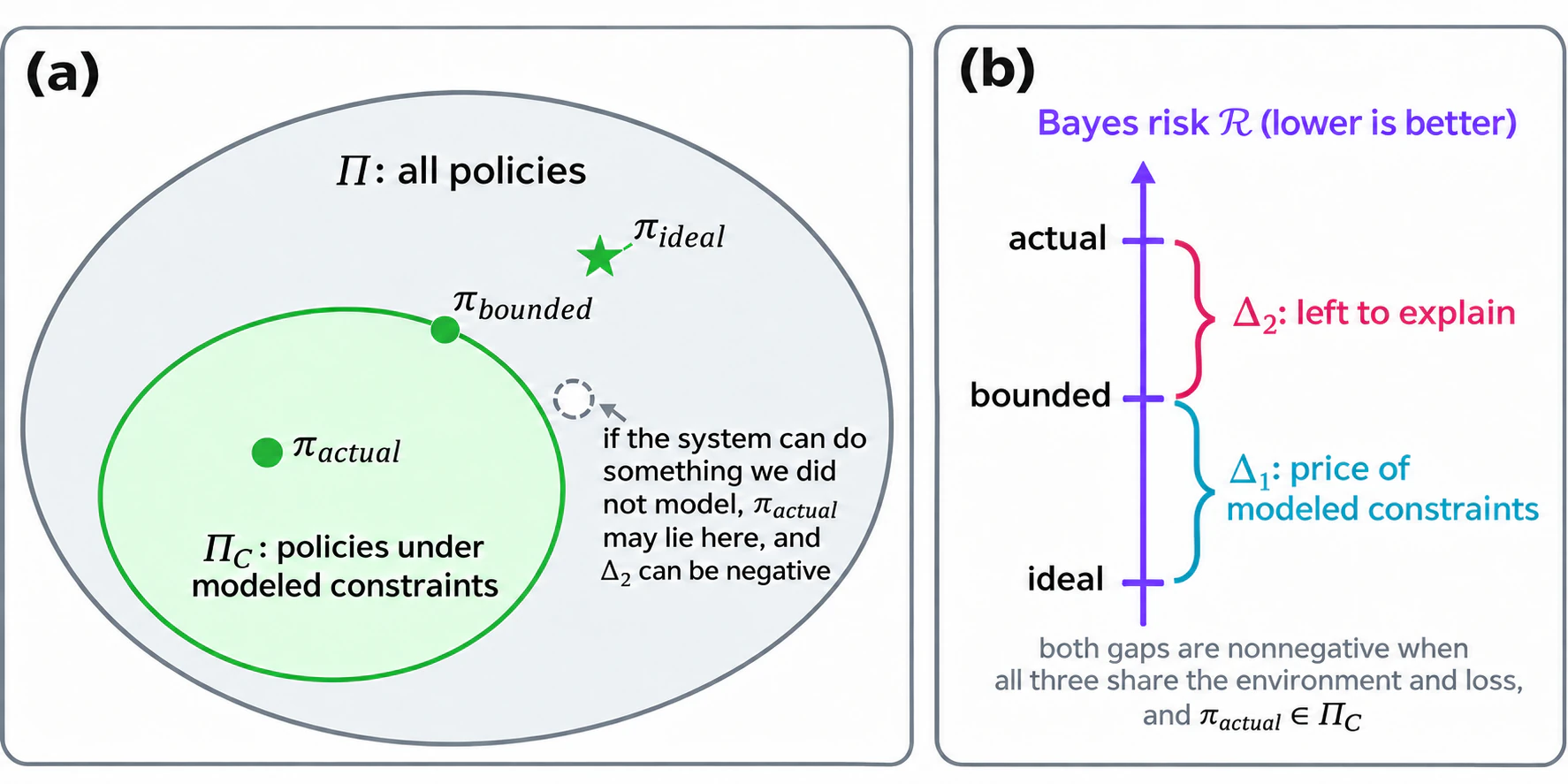
The ideal agent sees exactly the same $x$ as the system. It has no extra information; it is only free of the modeled limits on internal noise, time, and compute. Its own risk $\mathcal{R}(\pi_{\text{ideal}})$ is not zero either: that floor is set by how much information $x$ carries, and no system gets past it. The bounded agent is the best anything could do under those limits. If the actual policy lies inside $\Pi_C$, the gap to the ideal splits in two:
$$\mathcal{R}(\pi_{\text{actual}}) - \mathcal{R}(\pi_{\text{ideal}}) \;=\; \underbrace{\mathcal{R}(\pi_{\text{bounded}}) - \mathcal{R}(\pi_{\text{ideal}})}_{\Delta_1 \,\geq\, 0} \;+\; \underbrace{\mathcal{R}(\pi_{\text{actual}}) - \mathcal{R}(\pi_{\text{bounded}})}_{\Delta_2 \,\geq\, 0}.$$
$\Delta_1$ is the price of the constraints we modeled: how much worse any system must do once it has this much noise, this little time, this much compute. $\Delta_2$ is everything else. Learning may be unfinished, the algorithm may be approximate, the loss hypothesis may be wrong, or there may be a constraint we forgot. The efficiency of Section 1.3 was an early version of this comparison.
“Bounded” here means the best policy within a constrained class, the bounded optimality of Russell and Subramanian (Section 1.3), close to computational rationality [64] and resource-rational analysis; satisficing in Simon’s sense [65] is a different use of the word.
Fig. 10. Two references, two gaps. The ideal policy is best with the system’s information; the bounded policy is best under the modeled constraints. Δ₁ measures the price of those constraints, and Δ₂ what remains to explain. The nonnegative-gap interpretation requires a shared environment and loss and an actual policy inside ΠC. Outside ΠC, Δ₂ can be negative, but need not be.
Interpreting both gaps as nonnegative requires that all three policies share the environment and the loss, and that the actual policy lie inside $\Pi_C$. If the system can do something our constraint model rules out, $\pi_{\text{actual}}$ falls outside $\Pi_C$, and $\Delta_2$ can come out negative, which is itself informative: the constraint model is wrong.
Combining the ideal observer with a bounded reference in one comparison is what turns a gap into a clue. A large $\Delta_1$ says the task is hard under these constraints, and the system may be doing about as well as anything could. A large $\Delta_2$ says something is left to explain. For a system we train ourselves, the split maps directly onto two kinds of intervention. $\Delta_1$ is the price of the parameters and compute we chose, and scaling up shrinks it. $\Delta_2$ is optimization that did not reach the best policy within the constraints, an approximate algorithm, a wrong loss hypothesis, or a constraint we left out; scaling does not shrink it, and what has to change is the training and the objective. Which part of the gap is large decides where to push.
Scaling laws measure exactly $\Delta_1$. Hoffmann et al. (2022) [66] fit the test loss of language models as $E + A/N^{\alpha} + B/D^{\beta}$: $E$ is the floor no model gets past, corresponding to $\mathcal{R}(\pi_{\text{ideal}})$, and the other two terms are the price of parameters and of data, slices of $\Delta_1$ along those two axes. Three things differ. First, scaling laws measure the gap under the training loss $\ell$, not under the task $J$. Second, $E$ is an asymptote fitted within one model family, so a limit shared by the whole family is invisible there; the ideal reference of a normative model comes from outside the family. Third, scaling laws count the amount of data as a constraint, inside $\Delta_1$; in the setup of this section, too little data belongs to the unfinished learning of $\Delta_2$.
Such a move is not always legitimate. Whenever $\Delta_2$ shows up, you can invent a constraint that moves it into $\Delta_1$, and with enough inventions every system looks optimal. There is one standard for whether a constraint belongs in $\Delta_1$: it needs evidence independent of the behavior it is meant to explain. Either it can be measured on its own, as sensory noise is measured in a separate task, or it can be changed, and the gap moves as predicted; scaling experiments do exactly this with parameters and data. A constraint that can be neither measured nor changed is a free parameter, and the gap it props up is still $\Delta_2$. And constraints are not the only thing that can be moved: the loss, the prior, and the constraints can trade off against one another. That is the subject of the next section.
### 3.3 · What else does it take to read an objective off behavior?
To analyze an intelligent system, all one can see is behavior: a trajectory, a set of decisions, a batch of data. Reading the objective off the behavior is the most direct idea, and it has a long tradition. Savage (1954) [67] proved that if a person’s preferences among gambles satisfy a few axioms, both their probability judgments about the world and their utility for the outcomes can be recovered from those preferences, and both are unique (the utility up to an affine transformation). That is exactly a prior and a loss fixed by behavior.
So, given a hypothesis about the objective, can it be tested directly against the observed behavior? It cannot, and Wald’s theory contains the reason.
Start with something harmless. For any $c > 0$ and any function $b(\theta)$, the loss $c\,L(\theta, a) + b(\theta)$ leads to exactly the same optimal policy as $L$. A loss is identified at most up to rescaling and a world-dependent offset.
The next problem is more serious. The Bayes decision depends on the prior and the loss only through their product in the posterior expected loss,
$$\int L(\theta, a)\, p(x \mid \theta)\, p(\theta)\, d\theta.$$
Multiply the prior by any positive function $g(\theta)$, renormalize, and divide the loss by $g(\theta)$: every decision stays the same. From choices alone, a world believed rarer but costlier cannot be told apart from one believed more common and cheaper. This trade needs the loss to be free. Restricting it to a function of the error $\theta - a$ alone rules this one out, but identification still depends on the data: with Gaussian noise, every symmetric loss that grows with the error predicts the same aim, which is why the pea-shooter experiment of Section 3.1 made the error distribution skewed. Noise, information limits, and objectives can trade off in similar ways. The deepest study of such trades is structural estimation in economics: in dynamic discrete choice models, the utility, the discount factor, and the distribution of the unobservables are not jointly identified, and some of them have to be fixed first [68].
Wald’s complete class theorem makes the point general. Under mild conditions, every admissible decision rule is a Bayes rule for some prior, or a limit of Bayes rules [4]. Almost any sensible behavior is therefore Bayes-optimal for *some* prior and loss. On its own, “the system is Bayesian” is closer to a language than to a hypothesis. Inverse reinforcement learning met the same fact early: an optimal policy is consistent with infinitely many rewards, the constant reward among them [69].
Savage’s theorem holds because it asks not for one observation but for preferences over all gambles, and because it assumes the utility does not vary with the state of the world. In Wald’s framework these are the two further things it takes to read an objective off behavior. First, the parts other than the objective, the environment and the constraints, must be fixed by evidence that does not come from the behavior, or limited by a structural assumption. Second, the behavior must be seen under different conditions: one condition gives one point, and only when conditions change do different hypotheses about the objective make different predictions. The best experiments have long worked this way. Ernst and Banks (2002) [70] measured visual and haptic noise separately, each in a single-cue condition, then predicted how people would weight the two cues when both were present, with no parameters left to fit. The prediction held. A normative model earns credibility in proportion to how few of its parameters were fit to the data it explains. Identification only up to an equivalence class is not a defeat either. Objectives in the same class predict the same behavior under every condition, so for prediction they are one hypothesis, just as Savage’s utility is fixed only up to an affine transformation. What has to be separated are the ones that predict differently, and that is what the second condition is for.
Celebrated results deserve the same scrutiny. Duffy et al. (2022) [71] reanalyzed the data of Körding and Wolpert (2004) [19] trial by trial and argued that the evidence for Bayesian learning comes from averaging, while individual trials show a recency bias. Whatever one concludes about that study, the episode makes the point: the way we analyze behavior can produce the appearance of optimality. Part IV takes this further, with a microprocessor, and shows why systems we train ourselves can meet both conditions above.
### 3.4 · Three questions
Put together, normative modeling comes down to three questions, for artificial systems and humans alike.
1. Where do objectives come from, and how do they shape learning and behavior?
2. What would an ideal system achieve, what is achievable under realistic constraints, and how does the actual system compare?
3. Which of these gaps reveal properties of the system, and which are artifacts of our assumptions or evaluation methods?
For brains, every question is hard. The task has to be inferred, the prior is learned and hidden, the constraints are partly unknown, and the objective evolution shaped is a guess. A single behavior can take years of careful experiments. For AI, nearly every one of those unknowns is something we wrote down, or could. That asymmetry is the subject of Part IV.
---
## Part IV · Why Normative Modeling Should Land in Modern AI
Normative modeling of brains is hard: almost nothing in the four parts is known for certain, and neither condition of Section 3.3 is easy to meet. Perception, motor learning, and cognitive neuroscience do it anyway, because nothing else answers the question of the objective (Part III), at the price of years of experiments per conclusion. In AI, much of this sits in our own code. This part argues that AI is well suited to normative modeling and in need of it: for models we train ourselves, both conditions can be met; the loop of Section 3.1, inferring what a trained system actually optimizes and going back to change the training, can be closed here, and repeated; and full access to the inside has not by itself produced understanding (Section 4.1). It ends by showing that this is already under way, sometimes under this name, more often not.
### 4.1 · Everything is accessible, so why is it still not understood?
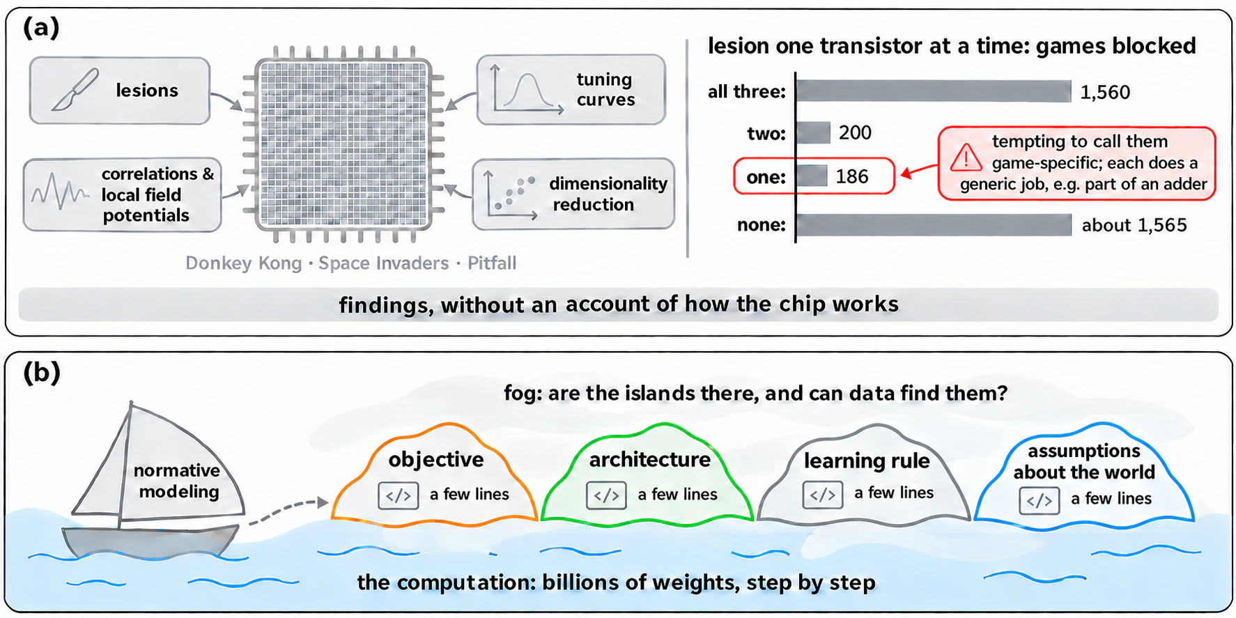
In “Could a Neuroscientist Understand a Microprocessor?” [72], two scientists who study brains applied the standard methods of their field to a chip that is fully known, to see whether the methods could recover how it works. They simulated the MOS 6502, the chip inside early home computers and game consoles, transistor by transistor, treated three games, Donkey Kong, Space Invaders, and Pitfall, as its behavior, and ran lesions, tuning curves, correlation analysis, and dimensionality reduction in turn. The methods did produce findings. Lesioning each of the 3,510 transistors found 186 whose removal stopped exactly one game. The authors point out that reading them as transistors specific to a game would be grossly misleading: each does a generic job, such as part of a full adder. The other methods found things too; dimensionality reduction picked up the clock and the read-write signal, and causal analysis found registers influencing the accumulator. But the authors conclude that this is nowhere near an understanding of how the processor works, and none of it approaches the description an engineer would give: registers, an instruction set, the fetch-and-execute cycle.
The result has an earlier precedent. Neuropsychology long treated double dissociation as evidence for modules: if one lesion impairs function A but not B and another impairs B but not A, then A and B are served by different parts. Plaut (1995) [73] trained a network to map spelling to meaning. Its structure is simple: a layer of spelling units, a layer of semantic units, a fully connected hidden layer between them, and a set of clean-up units that help the semantics settle; concrete and abstract words travel the same path through the same connections, and no part of the network is dedicated to either kind of word. After training, lesions at different locations left some networks worse on abstract words and others worse on concrete words: a double dissociation. The inference is direct. The network had no modules to begin with, so the dissociation cannot have been produced by modules. The damage was selective because the two kinds of word depend on the same connections to different degrees; concrete words have richer semantic features and tolerate different kinds of damage differently. Which function a lesion hurts says how much each task relies on those connections, not whom they belong to.
The result on the microprocessor is not an accident either; a short argument shows it had to appear. Think of the chip as a set of parts, each game using some of them, not all. As long as the three games do not use exactly the same parts, some part is used by only some of the games, and removing it breaks only those. The 186 transistors are the ones among them used by a single game. But “used by which games” is a property of this set of games, not of the part. Only when each function serves a fixed set of tasks does the usage label coincide with the function label. General-purpose hardware is exactly not like that: a transistor whose removal breaks only one game may be part of an adder, one the code of the other two games happens not to pass through. So from which functions disappear when a part is removed, one cannot infer that the part is the module responsible for them.
Today’s large neural networks are, in a sense, the microprocessor at scale. Every weight can be inspected, every activation recorded, every unit lesioned, every experiment rerun. Mechanistic interpretability has found real structure this way. One example is in vision. Olah et al. (2020) [74] found, in an image classifier, a unit that recognizes cars, assembled from window, body, and wheel detectors in the layer below, with the windows wired to its top and the wheels to its bottom. Rajaram et al. (2024) [75] automated the search: given a few dozen example images, their method extracts the circuit responsible for a concept, recovered the same car circuit, and found a text-detecting circuit in CLIP; cutting it raised the model’s accuracy under typographic attacks, such as the word “green” written on a red light, from 3% to 87%. Another example is in language models. Induction heads are a circuit of two attention heads: the first carries, to each position, the identity of the token just before it; the second uses that to find where the current token last appeared in the context and promotes the token that followed it as the next prediction, so that having seen “A B” earlier, it predicts B on seeing A again. This circuit is thought to be one of the main mechanisms of in-context learning [76]. These findings, however, live at the level of units and small circuits. A higher-level explanation of why a frontier model gives the answer it gives, one that unifies many such parts, is something mechanistic interpretability has made little progress toward. The microprocessor result suggests why: access alone does not tell us where the explanation should sit.
Where should the explanation sit? This essay’s answer: in the things that generate the computation. A running intelligent system carries out a computation over billions of weights, but few things generate that computation: the objective, the architecture, the learning rule [77], and a few top-level assumptions the system holds about the structure of the world. Each takes a few lines of code or a few equations to write down; each stays fixed while the computation runs, yet decides what the computation becomes, and predicts behavior in conditions that never occurred in training; together they are far smaller than the running system. What explains a system is here, not in the computation itself. When Section 3.1 said that normative modeling decides what learning takes as given, these are what it meant.
To call these the explanation is to apply a standard: an explanation is a description far smaller than the system itself that still predicts the system’s behavior under new conditions [58]. For an intelligent system whose computation is very dense, the computation itself may have no such description at all. Marr (1977) [78] called this a Type 2 theory: a problem solved by the simultaneous action of many processes whose interaction is its own simplest description; a network that has learned to recognize objects is likely such a case, its millions of trained weights already being its most compact description [79]. The task, then, is to search for “islands of explanatory simplicity in a sea of computational complexity” [58]: the sea is the computation itself, the islands are the rules that generate it. Whether such islands exist for a given complex system is an empirical question.
Hierarchical Bayesian models in cognitive science explain a learner in just this way. Their question is how people learn so much from so little [80], and their answer is that the learner carries abstract knowledge arranged in levels: at the top, a few assumptions about what structure the world has; at the bottom, specific facts; and the top decides what can be learned from little data. To explain a learner is to write down its top-level assumptions, not to list everything it has learned.
Even where the “islands” exist, data may not let us find them: different objectives can produce the same behavior (Section 3.3), and different training histories can end in similar networks. Normative modeling is the discipline for working on islands in this “fog”: write down a candidate objective, derive what it predicts, and test it where the candidates disagree, which is the second condition of Section 3.3.
Fig. 11. (a) Neuroscience methods applied to a fully known microprocessor produce findings without recovering how the chip works. Lesion counts are summarized with approximately proportional bars; 1,560 and about 1,565 are visually equal at this scale. The 186 transistors whose removal blocks one game should not be read as game-specific mechanisms [72]. (b) Islands of explanatory simplicity in a sea of computational complexity (the analogy is from Kording [58]): the islands are what generates the computation, the objective, the architecture, the learning rule and the top-level assumptions about the world, each a few lines long; the fog stands for what data cannot settle. Both panels are original schematics.
### 4.2 · Where AI is more accessible than a brain
In AI the “fog” is thinner: among the things that produce the computation, the top-level assumptions the system has learned and the objective it actually pursues still have to be inferred (see the second point below), but the training loss, the data, the architecture, and the learning rule were written down by us. This is what the first condition of Section 3.3 is about. To read an objective off behavior, the parts other than the objective, the environment the system faces and the constraints it works under, cannot also be guessed from the same behavior; otherwise the prior, the constraints, and the loss trade off against one another and the inferred objective is not unique. Those parts have to be fixed another way, measured separately or known in advance. Compare, part by part, how far a brain and a trained model meet this condition.
| | Brain | Trained model |
| --- | --- | --- |
| Environment and data | Inferred from ecology and experiment | Logged: the training data are on disk |
| Objective | Inferred; evolution’s is a guess | The training loss $\ell$ is in the code |
| Architecture and constraints | Partly known, hard to change | Specified, and changeable at will |
| Learning rule | Largely unknown | A known optimizer with a known schedule |
| Interventions | Limited, often irreversible | Retrain, ablate, perturb, repeat |
| Replicates | One lifetime per individual | As many seeds and variants as compute allows |
The first four rows concern the first condition, the last two the second: only with intervention and repetition can behavior be watched under different conditions. The right column describes models we train ourselves. For someone else’s closed model, the data and the training details are out of view, and several rows fall back toward the left column.
Three things follow. First, normative explanations can be checked against ground truth. For a brain, nobody knows the true objective, so an inferred objective can only be tested against more behavior, never against the answer; hiding the truth, giving the analyst only behavior, and seeing how much comes back can only be a thought experiment in neuroscience. In AI it can be run: train a family of models whose objectives, data, and architectures differ in known ways, hide those choices from the analyst, give them only behavior, and ask how much they recover, the objective, prior, and constraints themselves or only an equivalence class of them. The cost is compute.
Second, the training loss is ours, but the trained policy does not necessarily act by it. The optimizer drives down $\ell$ on the training data, and that part holds no surprise; what training leaves behind is a policy, and under new conditions its behavior often looks like the pursuit of a different objective, the behavioral objective $L$ of Section 3.1. Section 4.4 gives an example: with the same loss, policies trained on task sets of different diversity behave like Bayesian estimators under two different priors and perform very differently on new tasks. So in AI, $L$ still has to be inferred from behavior.
Third, the loop of Section 3.1 can be run here in full, and repeated. Its first half is choosing the loss before training from what the task requires; its second half is inferring, after training, what the system actually optimizes, comparing that with what we wanted, and going back to change things. For a brain, the second half allows only slow and coarse interventions, and none can be repeated: education can change the objective but not the architecture, and no one can retrain the same person from scratch. For a trained model, every row of the table can be changed and the model retrained, and the split of Section 3.2 says which row: if the gap falls in the constraints, scale up; if it falls in the remainder, change the training and the objective. Testing a proxy reward against a gold reward, as in Section 2.3, is already one instance of this second half.
### 4.3 · The landing has already begun
A good deal of recent work already treats AI systems this way: write down the problem the system was trained to solve, derive the best behavior for that problem, and compare it with what the model does. Most of it does not use the name normative modeling. Grouped by the three questions of Section 3.4:
**Where do objectives come from, and how do they shape behavior?**
- **The training problem predicts failures.** McCoy et al. (2024) [81] proposed to understand language models through the problem they were trained to solve, next-token prediction on internet text. It follows that a system optimal for this problem will care about the probability of the answer, even when the task itself is deterministic. The prediction held. GPT-4 decoded a simple shift cipher correctly about 51% of the time when the answer was a high-probability sentence and about 13% when it was low-probability, and its accuracy spiked for rot-13, by far the most common shift online. This is the second half of the loop of Section 3.1: predict the behavioral objective $L$ from the training objective, then test it in new conditions.
- **Objective and constraints generate the candidate solution.** Networks trained to recognize objects turned out to predict responses in monkey visual cortex [82], and Richards et al. (2019) [77] named objectives, architectures, and learning rules as the three components for understanding brains. The arrow there points from AI to brains, but the logic is normative: specify the objective and constraints, let optimization find a solution, compare it with the system.
**How close to ideal?**
- **Meta-learning approaches Bayes-optimality.** Memory-based meta-learners trained on a distribution of tasks come to behave like Bayes-optimal agents for that distribution [83, 84]. The ideal reference here is the $\pi_{\text{ideal}}$ of Section 3.2, and what training shrinks is the distance to it.
- **In-context learning as inference.** In-context learning can be read as implicit Bayesian inference [85], and transformers trained to do linear regression in context approach the optimal least-squares estimator [86]. Raventós et al. (2023) [87] and Wurgaft et al. (2025) [88] take this furthest, computing both the ideal and the bounded reference; Section 4.4 works through their setting.
**Property of the system, or artifact of the analysis?**
- **Identifiability has limits.** Even with unlimited data, reward learning can recover the reward only up to an equivalence class, and which class depends on the behavior model the analyst assumes [89]. This is the conclusion of Section 3.3 in its AI form: until the parts other than the objective are fixed, the objective is not.
- **Predicting well is weak evidence of a world model.** A transformer trained on planetary orbits predicts trajectories accurately, yet when adapted to predict forces, the force law it implies looks nothing like Newton’s [90]. Intervening on internal representations gives stronger evidence: editing the board state inside a model trained on Othello moves changes its predicted moves in the way the edit implies [91]. The first test stays within the training conditions; the second creates a new one, and the difference is the second condition of Section 3.3.
- **Benchmarks can hide replay.** Vision-language-action models that score above 90% on a standard manipulation benchmark can fall to near zero when objects, initial states, instructions, or environments are perturbed [92]: much of the score came from replaying trajectories. A benchmark is a proxy for the task $J$, and this is the gap of Section 2.3 appearing on the evaluation side.
The warning at the end of Section 3.3 applies in AI as well: the way we analyze can produce appearances. An intervention can push a system outside its normal operating range, a probe can fail because the readout is wrong, and the same representation can be written in many equivalent coordinates. Claims about what a model “has” deserve the same scrutiny as claims about what a brain has.
### 4.4 · A worked example: in-context learning
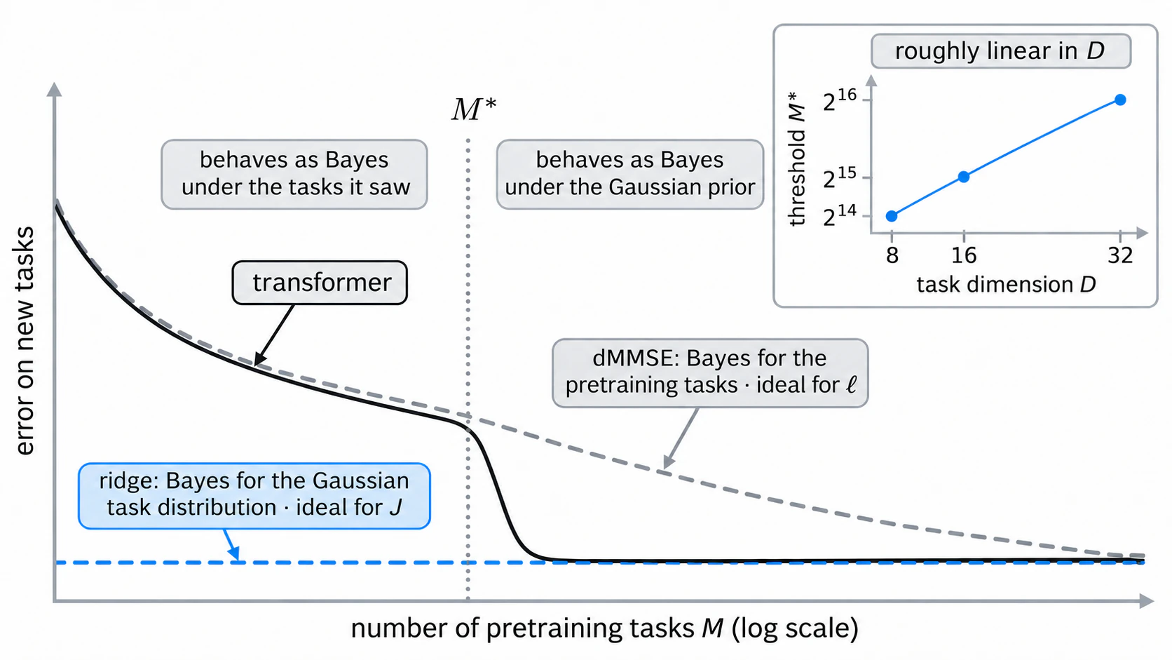
In-context learning on linear regression is small enough that every quantity in Part III can be computed. It is also the case in which the right column of the table in Section 4.2 holds in full: the environment, the loss, the architecture, and the data are all ours, so the first condition of Section 3.3 is met outright, and what remains is the second, watching behavior under different conditions. The setup follows Raventós et al. (2023) [87]. A task is a vector $w \in \mathbb{R}^D$. Inputs are $x_k \sim \mathcal{N}(0, I_D)$, and targets are $y_k = w^{\top} x_k + \varepsilon_k$ with $\varepsilon_k \sim \mathcal{N}(0, \sigma^2)$. A transformer reads $(x_1, y_1, \dots, x_{k-1}, y_{k-1}, x_k)$ and predicts $y_k$, trained with squared error. During pretraining, tasks are drawn uniformly from a fixed set of $M$ vectors $\{w^{(1)}, \dots, w^{(M)}\}$, each sampled once from $\mathcal{N}(0, I_D)$. At test time, tasks are fresh draws from $\mathcal{N}(0, I_D)$.
There are two natural references, both ideal in the sense of Section 3.2, limited only by the information in the context and not by capacity, but for two different environments. The first is optimal for the pretraining world, a uniform prior over the $M$ tasks it saw. Its estimate is a posterior-weighted average of those tasks:
$$\hat{w}^{\text{dMMSE}}_k \;=\; \sum_{i=1}^{M} \frac{\exp\!\Big(-\frac{1}{2\sigma^2} \sum_{jFig. 12. One loss, two behavioral objectives. With few pretraining tasks, a transformer trained on in-context linear regression behaves like the Bayes estimator for its pretraining tasks (dMMSE) and fails on new tasks. Past a task-diversity threshold, it behaves like ridge regression, the Bayes estimator for the full Gaussian task distribution. dMMSE and ridge are the ideal references for the training loss $\ell$ and the task evaluation $J$ respectively (Section 3.2). Inset: the threshold grows roughly linearly with dimension. (Image source: redrawn after Raventós et al. [87].)
Now run the three questions.
**What objective does the behavior reflect?** All three objectives of Section 3.1 can be written down here. The training loss $\ell$ is the same on both sides of the threshold: squared error on the next target, over the $M$ pretraining tasks. The task evaluation $J$ is prediction error on new tasks from the Gaussian world. The behavioral objective $L$ differs: on the left the model acts as Bayes under a discrete prior, on the right as Bayes under a Gaussian prior. Same loss, different objective, and the data decided which.
**Ideal, bounded, actual?** First, which ideal? $\ell$ is defined on the $M$ tasks, and its ideal is dMMSE; $J$ is defined on the Gaussian world, and its ideal is ridge. Below the threshold the model sits close to the ideal of $\ell$ and far from the ideal of $J$: the gap between $J$ and $\ell$ from Part II, in a case where it can be computed. Measured against ridge, that gap shrinks as $M$ grows, in the way predicted, so $M$ passes the test of Section 3.2 for a constraint that may be counted in $\Delta_1$: it can be changed, and the gap moves with it. The gap is the price of the data, and the row of the table to change is the data. Above the threshold the gap runs the other way. Measured in the pretraining environment against dMMSE, the model’s risk is higher, a $\Delta_2 > 0$, and this is the gap we want, since it buys generalization under $J$. Which sign a gap has, and what it means, depends on the environment and loss it is measured under; when the three policies do not share one environment, $\Delta_2$ has no fixed meaning, which is what the condition in Section 3.2 is for. It also bears out the second point of Section 4.2: the optimizer drives down $\ell$, the trained policy need not act by it, and here acting otherwise is better. For a bounded reference, Wurgaft et al. (2025) [88] treat the candidate strategies as Bayesian predictors and give complexity a price. The resulting trade-off between fit and complexity predicts when during training the model switches strategies, and the time it takes to move toward memorization grows superlinearly with task diversity. This is a bounded reference in the sense of Section 3.2, the best predictor once complexity costs something, and the price of complexity passes the same test as $M$: it is not a free parameter, because it predicts the timing of the switch, and the timing moves with task diversity as predicted.
**Property or artifact?** This is the setting where the check against ground truth from the first point of Section 4.2 is cheapest. Train models across a grid of $M$, $D$, and training lengths. Hide the grid. Give an analyst only each model’s predictions on probe sequences, and ask which prior it acts as if it uses and where its threshold lies. Then check the answers on held-out conditions: new tasks, longer contexts, shifted input distributions. I would like to see this done systematically, because it would tell us how far behavior alone can take us when the answer is known.
Frontier models are harder for a definite reason: the first condition weakens. For someone else’s model the data are out of view, the environment and the prior have to be guessed, and the references cannot be computed. Normative modeling there falls back from computing a reference and comparing to generating hypotheses and testing them by intervention. The logic is unchanged; what changes is how much can be settled.
### 4.5 · Possible objections
Three objections share one answer: normative modeling deals with what comes before a method (Section 3.1), that is, what objective the method should work toward, under what constraints, and how to test it. So it does not compete with these methods.
**“Isn’t this just Bayesian modeling?”** Normative models are often Bayesian, but by the complete class theorem [4] almost any reasonable behavior is Bayes-optimal for some prior and loss. The content of a normative model is not in the label but in what it fixes: which environment, which constraints, which loss, and which new condition is used to test them.
**“Why not just do mechanistic interpretability?”** Mechanism says how a computation is carried out; a normative account says why this computation. In Marr’s levels the first sits at the algorithmic and implementational levels, the second at the computational level, and they answer different questions. They also need each other: a circuit is easier to find and to name when you know what it is for (Section 4.1), and a claim about internal objectives eventually has to be checked against mechanism.
**“Doesn’t the bitter lesson say to keep human analysis out?”** Sutton (2019) [93] stresses not writing human knowledge into a system’s algorithms, and using instead general methods that scale with computation to search and to learn. Normative modeling works on the part the lesson does not touch: what objective the system should search and learn toward. Scaling up compute and data alone is the same case: scale shrinks the part of the gap caused by the constraints, $\Delta_1$ (Section 3.2), and not $\Delta_2$; when the behavioral objective differs from what we want, more optimization only widens the gap (Figure 7). One reason scale looks sufficient in practice is that people adapt to the system (Section 5.2).
---
## Part V · Objectives That Evolve
So far the objective has appeared in two places: chosen by us when building a system, inferred by us when explaining one. Changing it has also been our job, between runs. In the systems now being built, that step is starting to pass to the systems themselves: reward models are retrained, judges are swapped, agents write rewards for other agents. This last part asks what normative modeling has to say about objectives that evolve.
### 5.1 · Hierarchical loops in the evolution of intelligent systems
Any update in a learning system is made while other things are held fixed. A gradient step changes the parameters while the loss, the data, and the architecture stay put; to judge a loss, you have to train the parameters under it and look at the result; to judge an architecture, you have to train it, perhaps under several losses. So updates come in an order: a thing can be judged only after everything held fixed for it has been run. In that order, updates nest into loops, and one sample for an outer loop costs a full run of everything inside it. Wherever a system changes itself by its results, this nesting is present, and several fields have found it on their own: Ashby’s (1952) [94] ultrastable system has a slow loop watch a fast one and change its parameters only when the fast loop fails to keep its essential variables within bounds; hyperparameter optimization and meta-learning write the same structure as bilevel optimization, where the outer objective is defined by the solution of the inner problem; in hierarchical Bayesian models the hyperprior has to be learned from many tasks, each of which gives it one sample [95]; and in the brain, slow dopamine-driven learning trains a fast learner inside prefrontal cortex [96].
How many loops is a choice. Simon (1962) [97] observed that complex systems are almost always nearly decomposable, with strong interactions inside components and weak ones between them, so that different regularities change on different timescales; a quantity should be updated on the timescale on which it changes, and a world with so many separable timescales deserves that many loops. This essay uses three, because the four parts of Section 3.1 fall into three groups by who changes them: the policy, the weights, solved by training with the loss given; the loss and the criterion, the objective, changed today by post-training, reward modeling, and the hand work researchers do between runs, the second half of the loop of Section 3.1; and the world and the policy class, the data and the architecture, changed by architecture search and by the field’s decisions about what to pretrain next. In animals the three correspond roughly to learning within a lifetime, the tuning of drives on the timescale of development, and evolution. The loops can be merged or split; only the order is fixed. These are not Marr’s levels: Marr’s are three descriptions of one computation at one moment, these are a matter of what is held fixed for what.
The order sets the evidence. The farther out a loop, the more a sample costs, so the fewer and noisier its samples, and the stronger the evidence each update should require. For a brain this is the extreme case: a lifetime yields one sample of how well a set of drives served an individual, and a species yields one sample of an architecture. Most of today’s machine learning lives in the innermost loop; the outer two are still mostly run by people. What to take from this is a question: how much evidence should each kind of update require?
Few samples need not mean slow learning. Statistics has more curses than blessings: the curse of dimensionality says that within one level, the more parameters, the less the samples suffice [23], and Section 5.3 meets the optimizer’s curse. Across levels there is a result in the other direction, the blessing of abstraction [98]: abstract knowledge at the top can be learned faster than specific knowledge below it, because the hypotheses at the top are few and every specific task below supplies evidence for them. A child learns the rule that kinds are sorted by shape before learning the shape of each kind [95]. In terms of loops: the outer loop has few samples, but it also has little to settle, and what it settles is abstract; this is one reason the islands of Section 4.1 can be found at all. So the real difficulty of an outer loop is not the number of its samples but whether they are independent of what it judges, which is the subject of Section 5.3.
Automation makes the question of evidence pressing. Part II showed that the loss looks like all of modeling because the step after it was automated and the rest was set to defaults, and the same pressure is now moving outward. Language models write reward functions for robots as code [99], and architecture search and automated research push the slowest loop toward machines as well. Each step makes outer updates cheaper. It does not make the evidence for each update any less scarce. Faster outer loops mean more updates judged against the same evaluations, and more chances to fit the evaluations themselves: the reward hacking of Section 2.3, moved to the outer loops.
Fig. 13. Three loops. The four parts of Section 3.1 grouped by who changes them: the weights, changed by training, move fastest; the loss and criterion, that is, the objectives, more slowly; data and architecture slowest. One sample for an outer loop costs a full run of everything inside it, so the outer loops have few samples; but they also have little to settle, and the real difficulty is whether the evidence is independent (Section 5.3). Automation is beginning to run the outer loops too.
### 5.2 · Good evolution and bad evolution
Objectives change, and whether a change was good can only be judged by its outcome: after the environment moves, is the system better or worse at the task we care about? By that standard, good evolution has a few marks. The objective changes when the environment does; each change is checked before the next begins; and what the check rests on is something the system cannot influence. Bad evolution is the reverse: the objective fits an environment that has already drifted from the task, the check rests on exactly what the system can influence, and so the metric keeps improving while the task is no longer served. The difference is not how hard the system optimizes but what evidence the objective is changed on.
Nature has both. More than half a billion years ago, *Anomalocaris* was the top predator of Cambrian seas [100], its spiny frontal appendages built for grabbing soft-bodied prey [101]. Over the following tens of millions of years, prey grew hard shells or burrowed into the sediment, plankton diversified enormously, and the raptorial radiodonts disappear from the fossil record; their filter-feeding relatives changed what they ate and persisted, among them *Aegirocassis*, more than two meters long [102, 103]. The record supports this only as one reading, but as a story it fits: one line kept an objective fitted to a world that was going away, the other changed its objective with the world.
The accumulation of frontier models over the past few years has followed the good path. They first established themselves in domains where answers can be checked: a program runs or it does not, a proof holds or it does not. Then they turned each mastered domain into a tool for the next: code to write rewards and build environments, simulation to train for the physical world, until by 2026 general-purpose models could control robot arms directly from camera images, reliably on simple pick-and-place and still poorly on precise manipulation [104, 105]. Each level was checked before the next began, and the checkers, compilers, proof checkers, and the physical world, are not under the model’s influence.
The same models can also become *Anomalocaris*. A model trained against benchmarks learns the benchmarks. An agent rewarded by tests can learn to satisfy the tests in ways nobody intended [49]. A model trained repeatedly on its own outputs loses the tails of the distribution it started from [106]. Each is an objective fitted to an environment that has drifted from the one we care about: the training loss $\ell$ keeps improving while the task $J$ is no longer served. The difference lies in the checker: benchmarks, tests, and the model’s own outputs are all things the model can influence.
The environment changes, and the environment includes us. Biology calls this niche construction: organisms alter their environment and are then selected by the environment they altered [107]. The size of doors, the width of roads, writing, and social habits are niches that people built; none is optimal for the task, but once built, whoever comes next has to fit it. Humanoid robots follow from the same logic: asked in the abstract, the best form for a job is rarely humanoid, but the environment has already been shaped by human bodies, and once door handles, stairs, and tools are written into the constraints, the bounded optimum leans humanoid. The same thing happens between us and our models, in the other direction: we change our prompts, our workflows, and our benchmarks to suit what a model is good at. The gap then closes from both ends, training moving $L$ toward $J$ and adaptation moving $J$ toward $L$. So when judging whether an objective should change, it matters whether the environment really changed or we accommodated the system.
Fig. 14. Good and bad evolution. (a) An ecological contrast between the Cambrian predator Anomalocaris and the Early Ordovician filter feeder Aegirocassis, used as an analogy for changing objectives, not a demonstrated ancestor–descendant sequence. The two animals are drawn to the same scale, with approximate body sizes; Aegirocassis is shown at a little over two meters, not at a claimed maximum size. Light gray marks conjectural parts. (b) Models turn checkable domains into tools for the next domain, each step checked by something the model cannot influence; the red side path is the case where the checker can be influenced.
### 5.3 · When should an objective change?
Three questions follow, and normative modeling gives each one a handle.
**When.** An objective is outdated when behavior that is optimal under it stops serving the task. In the notation of Section 3.1, the gap between $J$ and $\ell$ has opened, and it can open from two sides. The world may have moved: $J$ changed while $\ell$ did not, and behavior optimal under $\ell$ no longer serves $J$. *Anomalocaris* is this case; the objective was once right. Or the system may have moved: neither $J$ nor $\ell$ changed, but optimization pushed the policy into the region where the two diverge. The curve of Figure 7 and training against benchmarks are this case, an outer loop overfitting its evaluation. The symptom is the same and the remedy is not: in the first case $\ell$ should change to follow $J$; in the second it should not, and the fix is a different checker or less optimization. Section 5.2 adds a third: $J$ moved toward $L$ because we accommodated the system, and then the first thing to settle is whether $J$ really changed. The three signs introduced earlier help tell these apart: a proxy that keeps improving while an independent evaluation stalls or falls (Figure 7) is the second; a gap that does not shrink when the constraints are relaxed sits in $\Delta_2$, which says the problem is in the training or the objective itself, not in the constraints (Section 3.2); predictions that hold in the training conditions and fail in new ones (Section 4.3) is the first.
A system that changes its own objective turns “when” into a different question. It judges whether the objective is outdated by an evaluation it computes itself, and that evaluation is something it can influence: if it wants to change the objective, it can make the evaluation say the objective is outdated. For such a system, whether the objective is outdated cannot be settled by its own training signal, only by a $J$ it cannot reach. The direction of the risk also reverses: when people run the outer loop, the danger is that the objective changes too slowly; when the system runs it, the danger is that it changes too easily.
**How fast.** The outer loop has few samples, but Section 5.1 showed that this is not the main constraint. The principle there is that a quantity should be updated on the timescale on which it changes. The true value of the objective changes on the timescale of $J$, so changing the objective has two speed limits: no faster than $J$ actually moves, and no faster than independent evidence arrives. Automation lowers the cost of proposing a change and moves neither limit. The second can be put in numbers: comparing $K$ candidates on the same evaluation inflates the winner’s score by about $\sigma\sqrt{2\ln K}$ on average, more candidates and fewer evaluations meaning more inflation; this is the optimizer’s curse [108]. Reusing a holdout set adaptively can destroy its validity. The reusable holdout of Dwork et al. (2015) [109] limits the damage: it answers from the training data unless the holdout disagrees by more than a noisy threshold, so each query reveals little about the holdout. A system that revises its own objective is an adaptive analyst of its own evaluations, and inherits both problems.
**On what evidence.** On evidence the system cannot influence, the standard that separated good evolution from bad in Section 5.2. Its basis is in the structure of Section 5.1: what judges a loop cannot come from that loop itself, which is what Ashby meant by placing the essential variables outside the fast loop; the first condition that Section 3.3 put to the analyst is the other face of the same fact. Checkers can be ranked by independence. The physical world, compilers, and proof checkers are the hardest; a held-out human evaluation sits in the middle, and loses a little independence with each use, which is what the reusable holdout manages; benchmarks and the model’s own outputs are the softest, because the model can influence them. In practice this means being explicit about which evaluations are used to propose a change and which to test it, which parts of the pipeline the system can touch, and when an outside check is required. One structural fact remains. No evidence is independent absolutely, only one level above what it judges. The checker of the outermost loop has no further level outside it, only us. So staying open to correction from outside is not a virtue but a structural requirement of the outermost loop, and the fact that evaluators also err only tightens it.
### 5.4 · What is still open
Wald named two choices that mathematics cannot make: the loss, and how to aggregate over what is unknown. For most of the eighty-odd years since, people made those choices and mathematics did the rest. Deep learning handed the solving that follows the choice of loss to machines, and set much of the problem to defaults. Normative modeling, grown in the study of perception and action, treats the same choices as hypotheses about a system, and tests them.
AI systems are getting harder to explain from the inside; they are starting to make these choices themselves, and whether those choices are right cannot be judged by evidence they can influence; and their objectives, data, and architectures are almost entirely in our hands. That is why I think normative modeling should land in AI. It is the discipline that asks what a system is optimizing, how far that is from what it could achieve, and whether our answers describe the system or our methods. The same three questions apply when building one. The long-term goal is a system that recognizes when its objective is outdated and revises it using evidence it cannot manipulate, while staying open to correction from outside.
Some questions I would most like to see answered:
1. **How much can behavior alone recover?** With the objective, data, and architecture known but hidden from the analyst, which parts of a system’s objective, prior, and constraints can an analyst identify, and which only up to an equivalence class?
2. **Which gaps can scale close?** Does locating a gap relative to the ideal and bounded references predict which intervention helps: more capacity, different data, or a different objective?
3. **Do diagnoses travel?** Does a diagnosis made in one condition predict the effect of an intervention in another, or does each new condition need a new model?
4. **Can a system be trusted to judge that its own objective is outdated?** How fast, and on what evidence, should the objective change when the system can influence its own evaluations?
---
Cited as:
> Zhang, Xiao. (Nov 2026). Where objectives come from: Why AI needs normative modeling. *xzhang.art*. https://xzhang.art/NLF/
```
@article{zhang2026objectives,
title = "Where Objectives Come From: Why AI Needs Normative Modeling",
author = "Zhang, Xiao",
journal = "xzhang.art",
year = "2026",
month = "Nov",
url = "https://xzhang.art/NLF/"
}
```
---
## References
1. Neyman, J., and E. S. Pearson. “On the problem of the most efficient tests of statistical hypotheses.” *Philosophical Transactions of the Royal Society A*, 1933. [doi:10.1098/rsta.1933.0009](https://doi.org/10.1098/rsta.1933.0009)
2. Wald, A. “Contributions to the theory of statistical estimation and testing hypotheses.” *Annals of Mathematical Statistics*, 1939. [doi:10.1214/aoms/1177732144](https://doi.org/10.1214/aoms/1177732144)
3. Wald, A. “Statistical decision functions which minimize the maximum risk.” *Annals of Mathematics*, 1945. [doi:10.2307/1969022](https://doi.org/10.2307/1969022)
4. Wald, A. *Statistical Decision Functions*. Wiley, 1950.
5. Wald, A. “Sequential tests of statistical hypotheses.” *Annals of Mathematical Statistics*, 1945. [doi:10.1214/aoms/1177731118](https://doi.org/10.1214/aoms/1177731118)
6. Wald, A. *Sequential Analysis*. Wiley, 1947.
7. Wald, A., and J. Wolfowitz. “Optimum character of the sequential probability ratio test.” *Annals of Mathematical Statistics*, 1948. [doi:10.1214/aoms/1177730197](https://doi.org/10.1214/aoms/1177730197)
8. Arrow, K. J., D. Blackwell, and M. A. Girshick. “Bayes and minimax solutions of sequential decision problems.” *Econometrica*, 1949. [doi:10.2307/1905525](https://doi.org/10.2307/1905525)
9. Casselman, B. “The legend of Abraham Wald.” *AMS Feature Column*, June 2016. [Link](https://www.ams.org/samplings/feature-column/fc-2016-06)
10. Wald, A. “A method of estimating plane vulnerability based on damage of survivors.” Statistical Research Group, Columbia University, 1943. Reprinted as CNA Research Contribution 432, Center for Naval Analyses, 1980. [DTIC ADA091073](https://apps.dtic.mil/sti/pdfs/ADA091073.pdf)
11. Mangel, M., and F. J. Samaniego. “Abraham Wald’s work on aircraft survivability.” *Journal of the American Statistical Association*, 1984. [doi:10.1080/01621459.1984.10478038](https://doi.org/10.1080/01621459.1984.10478038)
12. Peterson, W. W., T. G. Birdsall, and W. C. Fox. “The theory of signal detectability.” *Transactions of the IRE Professional Group on Information Theory*, 1954. [doi:10.1109/TIT.1954.1057460](https://doi.org/10.1109/TIT.1954.1057460)
13. Tanner, W. P., and J. A. Swets. “A decision-making theory of visual detection.” *Psychological Review*, 1954. [doi:10.1037/h0058700](https://doi.org/10.1037/h0058700)
14. Green, D. M., and J. A. Swets. *Signal Detection Theory and Psychophysics*. Wiley, 1966.
15. Tanner, W. P., and T. G. Birdsall. “Definitions of d′ and η as psychophysical measures.” *Journal of the Acoustical Society of America*, 1958. [doi:10.1121/1.1909408](https://doi.org/10.1121/1.1909408)
16. Harris, C. M., and D. M. Wolpert. “Signal-dependent noise determines motor planning.” *Nature*, 1998. [doi:10.1038/29528](https://doi.org/10.1038/29528)
17. Todorov, E., and M. I. Jordan. “Optimal feedback control as a theory of motor coordination.” *Nature Neuroscience*, 2002. [doi:10.1038/nn963](https://doi.org/10.1038/nn963)
18. Trommershäuser, J., L. T. Maloney, and M. S. Landy. “Statistical decision theory and the selection of rapid, goal-directed movements.” *Journal of the Optical Society of America A*, 2003. [doi:10.1364/JOSAA.20.001419](https://doi.org/10.1364/JOSAA.20.001419)
19. Körding, K. P., and D. M. Wolpert. “Bayesian integration in sensorimotor learning.” *Nature*, 2004. [doi:10.1038/nature02169](https://doi.org/10.1038/nature02169)
20. Ratcliff, R. “A theory of memory retrieval.” *Psychological Review*, 1978. [doi:10.1037/0033-295X.85.2.59](https://doi.org/10.1037/0033-295X.85.2.59)
21. Bogacz, R., E. Brown, J. Moehlis, P. Holmes, and J. D. Cohen. “The physics of optimal decision making: A formal analysis of models of performance in two-alternative forced-choice tasks.” *Psychological Review*, 2006. [doi:10.1037/0033-295X.113.4.700](https://doi.org/10.1037/0033-295X.113.4.700)
22. Gold, J. I., and M. N. Shadlen. “The neural basis of decision making.” *Annual Review of Neuroscience*, 2007. [doi:10.1146/annurev.neuro.29.051605.113038](https://doi.org/10.1146/annurev.neuro.29.051605.113038)
23. Bellman, R. *Dynamic Programming*. Princeton University Press, 1957.
24. Howard, R. A. *Dynamic Programming and Markov Processes*. Technology Press of MIT and Wiley, 1960.
25. Åström, K. J. “Optimal control of Markov processes with incomplete state information.” *Journal of Mathematical Analysis and Applications*, 1965. [doi:10.1016/0022-247X(65)90154-X](https://doi.org/10.1016/0022-247X%2865%2990154-X)
26. Sutton, R. S., and A. G. Barto. *Reinforcement Learning: An Introduction*, 2nd ed. MIT Press, 2018. [Link](http://incompleteideas.net/book/the-book-2nd.html)
27. Schultz, W., P. Dayan, and P. R. Montague. “A neural substrate of prediction and reward.” *Science*, 1997. [doi:10.1126/science.275.5306.1593](https://doi.org/10.1126/science.275.5306.1593)
28. Chow, C. K. “An optimum character recognition system using decision functions.” *IRE Transactions on Electronic Computers*, 1957. [doi:10.1109/TEC.1957.5222035](https://doi.org/10.1109/TEC.1957.5222035)
29. Chow, C. K. “On optimum recognition error and reject tradeoff.” *IEEE Transactions on Information Theory*, 1970. [doi:10.1109/TIT.1970.1054406](https://doi.org/10.1109/TIT.1970.1054406)
30. Duda, R. O., and P. E. Hart. *Pattern Classification and Scene Analysis*. Wiley, 1973.
31. Vapnik, V. N. *Statistical Learning Theory*. Wiley, 1998.
32. Russell, S., and P. Norvig. *Artificial Intelligence: A Modern Approach*. Prentice Hall, 1995.
33. Russell, S., and D. Subramanian. “Provably bounded-optimal agents.” *Journal of Artificial Intelligence Research*, 1995. [doi:10.1613/jair.133](https://doi.org/10.1613/jair.133)
34. Griffiths, T. L., F. Lieder, and N. D. Goodman. “Rational use of cognitive resources: Levels of analysis between the computational and the algorithmic.” *Topics in Cognitive Science*, 2015. [doi:10.1111/tops.12142](https://doi.org/10.1111/tops.12142)
35. Lieder, F., and T. L. Griffiths. “Resource-rational analysis: Understanding human cognition as the optimal use of limited computational resources.” *Behavioral and Brain Sciences*, 2020. [doi:10.1017/S0140525X1900061X](https://doi.org/10.1017/S0140525X1900061X)
36. Torralba, A., and A. A. Efros. “Unbiased look at dataset bias.” *CVPR*, 2011. [doi:10.1109/CVPR.2011.5995347](https://doi.org/10.1109/CVPR.2011.5995347)
37. Geifman, Y., and R. El-Yaniv. “Selective classification for deep neural networks.” *NeurIPS*, 2017. [arXiv:1705.08500](https://arxiv.org/abs/1705.08500)
38. Madras, D., T. Pitassi, and R. Zemel. “Predict responsibly: Improving fairness and accuracy by learning to defer.” *NeurIPS*, 2018. [arXiv:1711.06664](https://arxiv.org/abs/1711.06664)
39. Russakovsky, O., et al. “ImageNet large scale visual recognition challenge.” *International Journal of Computer Vision*, 2015. [doi:10.1007/s11263-015-0816-y](https://doi.org/10.1007/s11263-015-0816-y)
40. Deng, J., J. Krause, A. C. Berg, and L. Fei-Fei. “Hedging your bets: Optimizing accuracy-specificity trade-offs in large scale visual recognition.” *CVPR*, 2012. [doi:10.1109/CVPR.2012.6248086](https://doi.org/10.1109/CVPR.2012.6248086)
41. Bertinetto, L., R. Mueller, K. Tertikas, S. Samangooei, and N. A. Lord. “Making better mistakes: Leveraging class hierarchies with deep networks.” *CVPR*, 2020. [doi:10.1109/CVPR42600.2020.01252](https://doi.org/10.1109/CVPR42600.2020.01252)
42. Sagawa, S., P. W. Koh, T. B. Hashimoto, and P. Liang. “Distributionally robust neural networks for group shifts: On the importance of regularization for worst-case generalization.” *ICLR*, 2020. [arXiv:1911.08731](https://arxiv.org/abs/1911.08731)
43. Gneiting, T., and A. E. Raftery. “Strictly proper scoring rules, prediction, and estimation.” *Journal of the American Statistical Association*, 2007. [doi:10.1198/016214506000001437](https://doi.org/10.1198/016214506000001437)
44. Bishop, C. M. *Pattern Recognition and Machine Learning*. Springer, 2006.
45. Guo, C., G. Pleiss, Y. Sun, and K. Q. Weinberger. “On calibration of modern neural networks.” *ICML*, 2017. [arXiv:1706.04599](https://arxiv.org/abs/1706.04599)
46. Elkan, C. “The foundations of cost-sensitive learning.” *IJCAI*, 2001.
47. Elmachtoub, A. N., and P. Grigas. “Smart ‘predict, then optimize’.” *Management Science*, 2022. [doi:10.1287/mnsc.2020.3922](https://doi.org/10.1287/mnsc.2020.3922)
48. Ouyang, L., et al. “Training language models to follow instructions with human feedback.” *NeurIPS*, 2022. [arXiv:2203.02155](https://arxiv.org/abs/2203.02155)
49. Krakovna, V., et al. “Specification gaming: The flip side of AI ingenuity.” DeepMind blog, April 21, 2020. [Link](https://deepmind.google/discover/blog/specification-gaming-the-flip-side-of-ai-ingenuity/)
50. Gao, L., J. Schulman, and J. Hilton. “Scaling laws for reward model overoptimization.” *ICML*, 2023. [arXiv:2210.10760](https://arxiv.org/abs/2210.10760)
51. Manheim, D., and S. Garrabrant. “Categorizing variants of Goodhart’s law.” arXiv, 2018. [arXiv:1803.04585](https://arxiv.org/abs/1803.04585)
52. Bradley, R. A., and M. E. Terry. “Rank analysis of incomplete block designs: I. The method of paired comparisons.” *Biometrika*, 1952. [doi:10.2307/2334029](https://doi.org/10.2307/2334029)
53. Luce, R. D. *Individual Choice Behavior: A Theoretical Analysis*. Wiley, 1959.
54. Christiano, P., J. Leike, T. B. Brown, M. Martic, S. Legg, and D. Amodei. “Deep reinforcement learning from human preferences.” *NeurIPS*, 2017. [arXiv:1706.03741](https://arxiv.org/abs/1706.03741)
55. Ziegler, D. M., et al. “Fine-tuning language models from human preferences.” arXiv, 2019. [arXiv:1909.08593](https://arxiv.org/abs/1909.08593)
56. Ortega, P. A., and D. A. Braun. “Thermodynamics as a theory of decision-making with information-processing costs.” *Proceedings of the Royal Society A*, 2013. [doi:10.1098/rspa.2012.0683](https://doi.org/10.1098/rspa.2012.0683)
57. Rafailov, R., A. Sharma, E. Mitchell, C. D. Manning, S. Ermon, and C. Finn. “Direct preference optimization: Your language model is secretly a reward model.” *NeurIPS*, 2023. [arXiv:2305.18290](https://arxiv.org/abs/2305.18290)
58. Kording, K. “Why we systems neuroscientists should (usually) be quietists: The philosophical logic of NeuroAI.” Substack, October 19, 2026. [Link](https://kording.substack.com/p/why-we-systems-neuroscientists-should)
59. Marr, D. *Vision: A Computational Investigation into the Human Representation and Processing of Visual Information*. W. H. Freeman, 1982.
60. Anderson, J. R. *The Adaptive Character of Thought*. Lawrence Erlbaum Associates, 1990.
61. Kording, K. “The simple conceptual logic of normative models of behavior.” Substack, March 17, 2025. [Link](https://kording.substack.com/p/the-simple-conceptual-logic-of-normative)
62. Körding, K. P., and D. M. Wolpert. “The loss function of sensorimotor learning.” *Proceedings of the National Academy of Sciences*, 2004. [doi:10.1073/pnas.0308394101](https://doi.org/10.1073/pnas.0308394101)
63. Hubinger, E., C. van Merwijk, V. Mikulik, J. Skalse, and S. Garrabrant. “Risks from learned optimization in advanced machine learning systems.” arXiv, 2019. [arXiv:1906.01820](https://arxiv.org/abs/1906.01820)
64. Lewis, R. L., A. Howes, and S. Singh. “Computational rationality: Linking mechanism and behavior through bounded utility maximization.” *Topics in Cognitive Science*, 2014. [doi:10.1111/tops.12086](https://doi.org/10.1111/tops.12086)
65. Simon, H. A. “A behavioral model of rational choice.” *Quarterly Journal of Economics*, 1955. [doi:10.2307/1884852](https://doi.org/10.2307/1884852)
66. Hoffmann, J., et al. “Training compute-optimal large language models.” *NeurIPS*, 2022. [arXiv:2203.15556](https://arxiv.org/abs/2203.15556)
67. Savage, L. J. *The Foundations of Statistics*. Wiley, 1954.
68. Magnac, T., and D. Thesmar. “Identifying dynamic discrete choice processes.” *Econometrica*, 2002. [doi:10.1111/1468-0262.00306](https://doi.org/10.1111/1468-0262.00306)
69. Ng, A. Y., and S. Russell. “Algorithms for inverse reinforcement learning.” *ICML*, 2000.
70. Ernst, M. O., and M. S. Banks. “Humans integrate visual and haptic information in a statistically optimal fashion.” *Nature*, 2002. [doi:10.1038/415429a](https://doi.org/10.1038/415429a)
71. Duffy, S., J. Hertel, D. Igan, M. Pinheiro, and J. Smith. “On Bayesian integration in sensorimotor learning: Another look at Kording and Wolpert (2004).” *Cortex*, 2022. [doi:10.1016/j.cortex.2022.03.021](https://doi.org/10.1016/j.cortex.2022.03.021)
72. Jonas, E., and K. P. Kording. “Could a neuroscientist understand a microprocessor?” *PLoS Computational Biology*, 2017. [doi:10.1371/journal.pcbi.1005268](https://doi.org/10.1371/journal.pcbi.1005268)
73. Plaut, D. C. “Double dissociation without modularity: Evidence from connectionist neuropsychology.” *Journal of Clinical and Experimental Neuropsychology*, 1995. [doi:10.1080/01688639508405124](https://doi.org/10.1080/01688639508405124)
74. Olah, C., N. Cammarata, L. Schubert, G. Goh, M. Petrov, and S. Carter. “Zoom in: An introduction to circuits.” *Distill*, 2020. [doi:10.23915/distill.00024.001](https://doi.org/10.23915/distill.00024.001)
75. Rajaram, A., N. Chowdhury, A. Torralba, J. Andreas, and S. Schwettmann. “Automatic discovery of visual circuits.” arXiv, 2024. [arXiv:2404.14349](https://arxiv.org/abs/2404.14349)
76. Olsson, C., et al. “In-context learning and induction heads.” Transformer Circuits Thread, 2022. [Link](https://transformer-circuits.pub/2022/in-context-learning-and-induction-heads/index.html)
77. Richards, B. A., et al. “A deep learning framework for neuroscience.” *Nature Neuroscience*, 2019. [doi:10.1038/s41593-019-0520-2](https://doi.org/10.1038/s41593-019-0520-2)
78. Marr, D. “Artificial intelligence: A personal view.” *Artificial Intelligence*, 1977. [doi:10.1016/0004-3702(77)90013-3](https://doi.org/10.1016/0004-3702(77)90013-3)
79. Lillicrap, T. P., and K. P. Kording. “What does it mean to understand a neural network?” arXiv, 2019. [arXiv:1907.06374](https://arxiv.org/abs/1907.06374)
80. Tenenbaum, J. B., C. Kemp, T. L. Griffiths, and N. D. Goodman. “How to grow a mind: Statistics, structure, and abstraction.” *Science*, 2011. [doi:10.1126/science.1192788](https://doi.org/10.1126/science.1192788)
81. McCoy, R. T., S. Yao, D. Friedman, M. D. Hardy, and T. L. Griffiths. “Embers of autoregression show how large language models are shaped by the problem they are trained to solve.” *Proceedings of the National Academy of Sciences*, 2024. [doi:10.1073/pnas.2322420121](https://doi.org/10.1073/pnas.2322420121)
82. Yamins, D. L. K., H. Hong, C. F. Cadieu, E. A. Solomon, D. Seibert, and J. J. DiCarlo. “Performance-optimized hierarchical models predict neural responses in higher visual cortex.” *Proceedings of the National Academy of Sciences*, 2014. [doi:10.1073/pnas.1403112111](https://doi.org/10.1073/pnas.1403112111)
83. Ortega, P. A., et al. “Meta-learning of sequential strategies.” arXiv, 2019. [arXiv:1905.03030](https://arxiv.org/abs/1905.03030)
84. Binz, M., et al. “Meta-learned models of cognition.” *Behavioral and Brain Sciences*, 2024. [doi:10.1017/S0140525X23003266](https://doi.org/10.1017/S0140525X23003266)
85. Xie, S. M., A. Raghunathan, P. Liang, and T. Ma. “An explanation of in-context learning as implicit Bayesian inference.” *ICLR*, 2022. [arXiv:2111.02080](https://arxiv.org/abs/2111.02080)
86. Garg, S., D. Tsipras, P. Liang, and G. Valiant. “What can transformers learn in-context? A case study of simple function classes.” *NeurIPS*, 2022. [arXiv:2208.01066](https://arxiv.org/abs/2208.01066)
87. Raventós, A., M. Paul, F. Chen, and S. Ganguli. “Pretraining task diversity and the emergence of non-Bayesian in-context learning for regression.” *NeurIPS*, 2023. [arXiv:2306.15063](https://arxiv.org/abs/2306.15063)
88. Wurgaft, D., E. S. Lubana, C. F. Park, H. Tanaka, G. Reddy, and N. D. Goodman. “In-context learning strategies emerge rationally.” *NeurIPS*, 2025. [arXiv:2506.17859](https://arxiv.org/abs/2506.17859)
89. Skalse, J., M. Farrugia-Roberts, S. Russell, A. Abate, and A. Gleave. “Invariance in policy optimisation and partial identifiability in reward learning.” *ICML*, 2023. [arXiv:2203.07475](https://arxiv.org/abs/2203.07475)
90. Vafa, K., P. G. Chang, A. Rambachan, and S. Mullainathan. “What has a foundation model found? Using inductive bias to probe for world models.” *ICML*, 2025. [arXiv:2507.06952](https://arxiv.org/abs/2507.06952)
91. Li, K., A. K. Hopkins, D. Bau, F. Viégas, H. Pfister, and M. Wattenberg. “Emergent world representations: Exploring a sequence model trained on a synthetic task.” *ICLR*, 2023. [arXiv:2210.13382](https://arxiv.org/abs/2210.13382)
92. Zhou, X., Y. Xu, G. Tie, Y. Chen, G. Zhang, D. Chu, P. Zhou, and L. Sun. “LIBERO-PRO: Towards robust and fair evaluation of vision-language-action models beyond memorization.” arXiv, 2025. [arXiv:2510.03827](https://arxiv.org/abs/2510.03827)
93. Sutton, R. S. “The bitter lesson.” Incomplete Ideas, 2019. [Link](http://www.incompleteideas.net/IncIdeas/BitterLesson.html)
94. Ashby, W. R. *Design for a Brain*. Chapman & Hall, 1952.
95. Kemp, C., A. Perfors, and J. B. Tenenbaum. “Learning overhypotheses with hierarchical Bayesian models.” *Developmental Science*, 2007. [doi:10.1111/j.1467-7687.2007.00585.x](https://doi.org/10.1111/j.1467-7687.2007.00585.x)
96. Wang, J. X., et al. “Prefrontal cortex as a meta-reinforcement learning system.” *Nature Neuroscience*, 2018. [doi:10.1038/s41593-018-0147-8](https://doi.org/10.1038/s41593-018-0147-8)
97. Simon, H. A. “The architecture of complexity.” *Proceedings of the American Philosophical Society*, 1962. [JSTOR](https://www.jstor.org/stable/985254)
98. Goodman, N. D., T. D. Ullman, and J. B. Tenenbaum. “Learning a theory of causality.” *Psychological Review*, 2011. [doi:10.1037/a0021336](https://doi.org/10.1037/a0021336)
99. Ma, Y. J., et al. “Eureka: Human-level reward design via coding large language models.” *ICLR*, 2024. [arXiv:2310.12931](https://arxiv.org/abs/2310.12931)
100. Paterson, J. R., D. C. García-Bellido, M. S. Y. Lee, G. A. Brock, J. B. Jago, and G. D. Edgecombe. “Acute vision in the giant Cambrian predator *Anomalocaris* and the origin of compound eyes.” *Nature*, 2011. [doi:10.1038/nature10689](https://doi.org/10.1038/nature10689)
101. Bicknell, R. D. C., M. Schmidt, I. A. Rahman, G. D. Edgecombe, S. Gutarra, A. C. Daley, R. R. Melzer, S. Wroe, and J. R. Paterson. “Raptorial appendages of the Cambrian apex predator *Anomalocaris canadensis* are built for soft prey and speed.” *Proceedings of the Royal Society B*, 2023. [doi:10.1098/rspb.2023.0638](https://doi.org/10.1098/rspb.2023.0638)
102. Van Roy, P., A. C. Daley, and D. E. G. Briggs. “Anomalocaridid trunk limb homology revealed by a giant filter-feeder with paired flaps.” *Nature*, 2015. [doi:10.1038/nature14256](https://doi.org/10.1038/nature14256)
103. Potin, G. J.-M., P. Gueriau, and A. C. Daley. “Radiodont frontal appendages from the Fezouata Biota (Morocco) reveal high diversity and ecological adaptations to suspension-feeding during the Early Ordovician.” *Frontiers in Ecology and Evolution*, 2023. [doi:10.3389/fevo.2023.1214109](https://doi.org/10.3389/fevo.2023.1214109)
104. Menon, A., S. Machcha, S. Zou, T. K. Chan, and J. Chooi. “GPT-6 Astra on robotic manipulation.” Robocurve, September 4, 2026. [Link](https://openai.robocurve.org/gpt-6-astra/)
105. Zhang, W., et al. “An unexpected robot policy: Early evaluations of GPT-6 Astra on RoboDojo and beyond.” arXiv, 2026. [arXiv:2609.24170](https://arxiv.org/abs/2609.24170)
106. Shumailov, I., et al. “AI models collapse when trained on recursively generated data.” *Nature*, 2024. [doi:10.1038/s41586-024-07566-y](https://doi.org/10.1038/s41586-024-07566-y)
107. Odling-Smee, F. J., K. N. Laland, and M. W. Feldman. *Niche Construction: The Neglected Process in Evolution*. Princeton University Press, 2003.
108. Smith, J. E., and R. L. Winkler. “The optimizer’s curse: Skepticism and postdecision surprise in decision analysis.” *Management Science*, 2006. [doi:10.1287/mnsc.1050.0451](https://doi.org/10.1287/mnsc.1050.0451)
109. Dwork, C., V. Feldman, M. Hardt, T. Pitassi, O. Reingold, and A. Roth. “The reusable holdout: Preserving validity in adaptive data analysis.” *Science*, 2015. [doi:10.1126/science.aaa9375](https://doi.org/10.1126/science.aaa9375)