Normative Learning Framework
1 · Three Puzzles
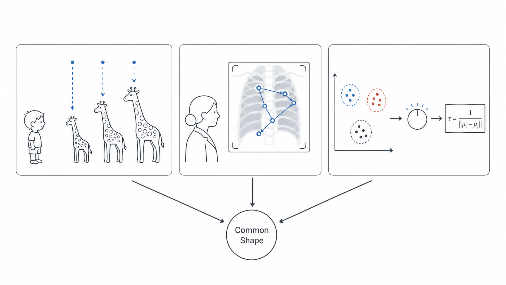
Puzzle 1. You have heard the old refrain: a two-year-old sees three giraffes and recognizes giraffes for the rest of her life, while modern networks need millions of examples and still fail under distribution shift. Look at any natural photograph and bird separates from sky before you decide to look at either. No one taught you this, and infants do it too. The standard explanation invokes “inductive bias,” and we move on. But this is more relabeling than answer. It pushes the question one step back without resolving it. What, exactly, is the visual system already representing, before any giraffe and before any photograph, that makes three examples sufficient and figure-ground separation automatic? Whatever it is, it was not learned from the data. It was waiting for the data.
Puzzle 2. Two radiologists look at the same chest X-ray. The senior finds the lesion in three seconds. The junior takes thirty and misses it. Both have seen thousands of cases. What, exactly, has the senior learned that the junior has not? It is not “more labels,” because they have seen the same labels. It is not “a better architecture,” because their visual systems are nearly identical. Their eyes simply move differently, and the difference is measurable, systematic, and shared across senior radiologists who have never met. Whatever they have converged toward, they have converged toward it together.
Puzzle 3. Modern deep learning is, in practice, an art of carefully tuned numbers. Temperature scales, margin parameters, learning-rate schedules: design choices, supported by ablation tables. Yet in 2019, working on face recognition, my collaborators and I found that one such hyperparameter, the softmax scale factor that practitioners had been tuning by hand for years, was not, in fact, free. Under a modest probabilistic assumption about the embedding geometry, it was determined: a closed-form function of statistics already present in the training batch. What had been tuned was a derived quantity all along. The discomfort this raises is general, not local. How much of what we treat as engineering art in deep learning is the visible shadow of a normative structure we have not yet articulated?
These three puzzles share a common shape. This research statement is about that shape, and about the framework I have developed to give it precise form.
2 · The Common Shape
2.0 · What the puzzles share
The three puzzles describe systems doing very different things. An infant forms a concept. A radiologist scans an image. A loss function is, in a sense, optimizing itself. Yet beneath the surface, they share a structural feature that current learning theory does not name.
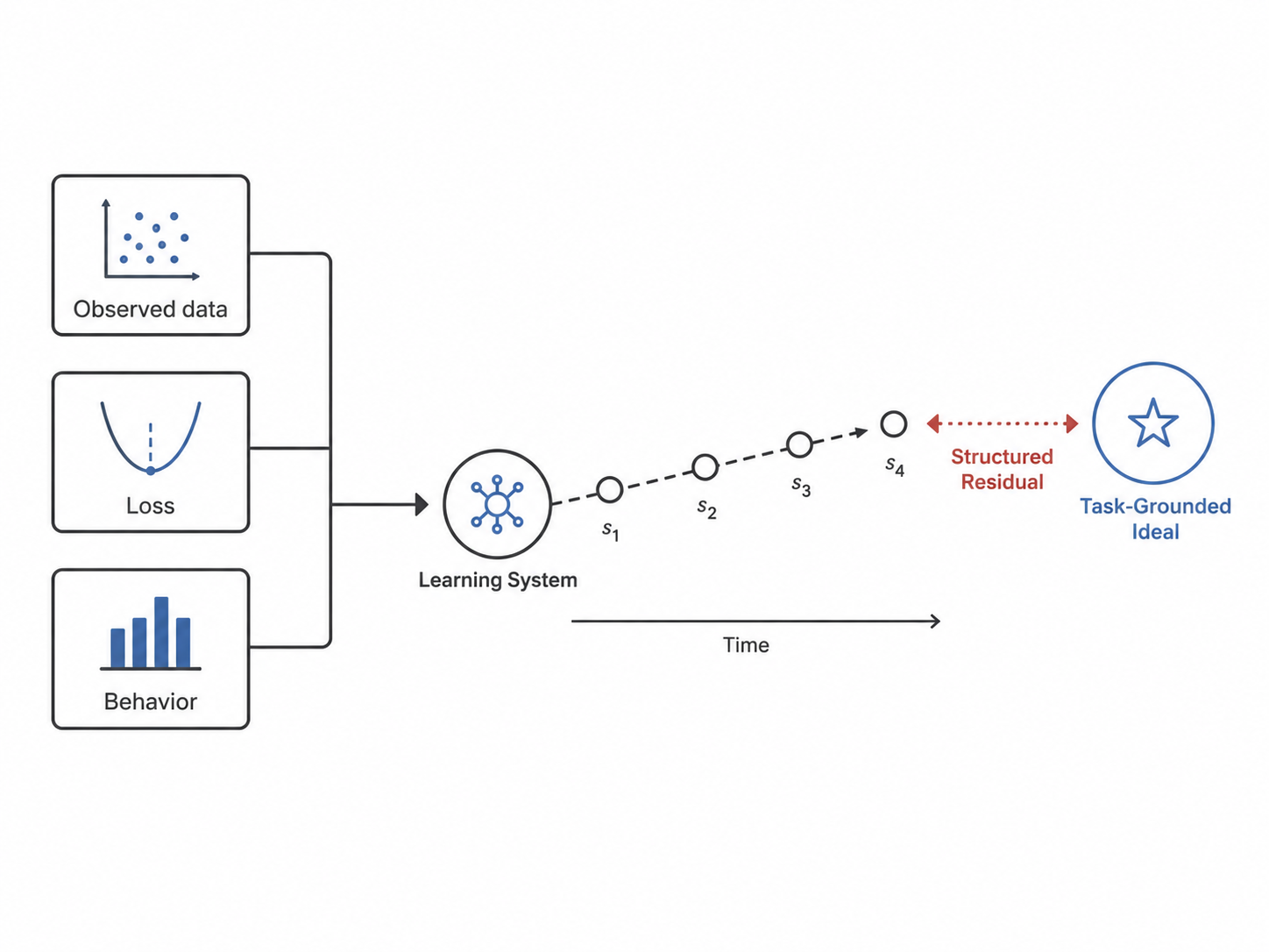
In each case, the system is approaching something that the data alone does not specify. The infant approaches a representation that makes giraffes intelligible long before she has met enough giraffes to define one. The radiologists approach a fixation policy that no individual could have invented and yet many independently reach. The softmax scale approaches a value that is not in the gradient signal but in the geometry the loss already presupposes. None of these targets is the loss being minimized. None is the label being fitted. All three are approached, and what is approached is not what is given.
This is the shape. It is not a metaphor. It is a precise structural claim: a learning system has a target that is logically prior to the data it sees, and the central question of any normative theory of learning is what that target is, where it comes from, and how systems get closer to it.
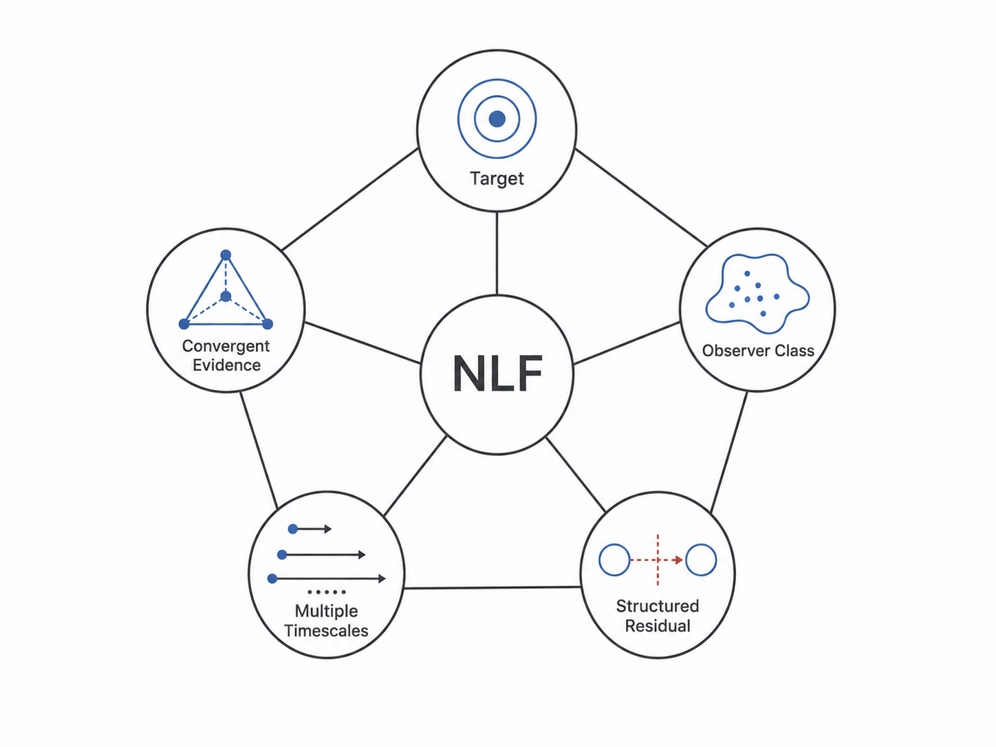
The Normative Learning Framework (NLF) is built around this claim. It rests on five commitments, each of which addresses a question the claim immediately raises: what is being approached (2.1), who is doing the approaching (2.2), how do we know the target is the right one (2.3), what does the gap mean when approach falls short (2.4), and over what timescales does approach unfold (2.5). The five commitments are not a list of features. They are the minimum set required to make the structural claim above operational.
2.1 · The target: a task-grounded ideal, not a chosen loss
Modern machine learning rarely asks where its loss functions come from. Cross-entropy, mean-squared error, contrastive objectives, margin-based softmax variants: these are presented as choices, defended by ablation tables, and refined by empirical comparison. The community has developed enormous skill in selecting losses but very little vocabulary for justifying them. We rarely say a loss is correct; we say it works.
This silence has a cost. When a system fails, we ask whether the architecture was wrong, whether the data was insufficient, whether optimization was unstable. We almost never ask whether the loss itself was the wrong object, because without an external reference, “wrong loss” is not a well-formed concept. A loss is just a loss. It is whatever someone decided to minimize.
The puzzles in 1 each violate this silence in a different way. The infant has no loss at all and yet forms representations that work. The radiologists do not share a loss and yet converge on the same policy. The softmax scale, when correctly analyzed, is not free to be tuned by ablation; it is fixed by the probabilistic structure of the embedding space. In each case, what governs the system’s behavior is not the loss on the surface but a deeper object: a target that the task itself, the data geometry, or the observer’s structure jointly specify, independently of any loss the engineer happens to write down.
NLF gives this target a name. It is the task-grounded ideal, written $w^{\ast}_T$ when the target is a representation and $\pi^{\ast}_T$ when it is a policy. The ideal is what the system should approach, given the structure of the task it is solving, the data it can access, and the observer it lives in. The loss, when chosen well, is an instrument for approaching this ideal. When chosen poorly, the loss approaches something else.
This shift, from loss as the object of study to ideal as the object of study, is the first commitment of NLF. It does not deny that losses matter. It denies that they are the right place to start. The right place to start is the question the AdaCos puzzle raised at the end of 1: how much of what we treat as engineering art in deep learning is the visible shadow of an ideal we have not yet articulated? The answer, NLF claims, is much more than the field currently admits.
2.2 · The actor: an explicit observer class
A task-grounded ideal does not hover in the abstract. It is approached by something: a network with a particular architecture, a brain with a particular cortical organization, a system with a particular budget of computation, memory, and time. What can be approached, and how closely, depends on what the actor is. Two systems pointed at the same ideal can be far from each other, and far from the ideal, for entirely structural reasons.
This is obvious in retrospect, but standard analyses of optimality often elide it. We ask whether a system is “Bayes-optimal” or “matches the ideal observer,” and we treat the answer as if it were a property of the system alone. But Bayes-optimality is defined relative to a hypothesis class, and the ideal observer is defined relative to a perceptual architecture. A convolutional network and a transformer, given the same data and the same loss, do not converge to the same place, and the difference is not noise. It is the visible footprint of two different observer structures meeting the same target.
NLF makes this dependence explicit. Every normative analysis is conducted relative to an observer class $\mathcal{F}$: the space of representations or policies a system can in principle realize, given its architecture, its data access, and its resource budget. The ideal $w^{\ast}_T$ is then defined not over an unbounded function space but over $\mathcal{F}$. The right question is not “is the system optimal?” but “how close is the system to the best element of $\mathcal{F}$, and how close is that best element to the unbounded ideal?” These two gaps have entirely different sources and entirely different remedies.
Making the observer class explicit also clarifies a question the puzzles raised but did not answer: where does the structure of the observer come from? The infant’s visual system is shaped by evolution and development long before any giraffe is encountered. The radiologists’ visual systems share an architecture but their fixation policies are shaped by years of practice. The softmax network’s observer class is shaped by the engineer who chose its layers. In each case, $\mathcal{F}$ is not given for free; it is itself the product of slower processes, a point 2.5 will return to.
2.3 · The justification: convergent evidence, not single fitting
A standard objection to any normative analysis is that it can be made to fit anything. Given a flexible enough family of objectives, one can almost always find a $w^{\ast}_T$ under which a system looks reasonable. Cognitive science has wrestled with this charge for decades under the heading of inverse rational analysis: if I can choose the utility function, I can rationalize any behavior. Normative claims, on this view, risk being unfalsifiable.
The objection is serious and must be addressed at the level of method, not rhetoric. NLF addresses it by refusing to let any single source of evidence determine the ideal. A proposed $U_T$, the formal object that defines $w^{\ast}_T$, is granted standing only when it is supported by convergent evidence from at least three independent directions.
The first is task-theoretic grounding: $U_T$ must be derivable from the formal structure of the task itself, in the sense that an unboundedly resourced reasoner with full access to the task’s specification would compute it. This is the criterion at work when we say that the Bayes classifier is the right ideal for binary classification under 0-1 loss, regardless of which dataset we happen to be looking at.
The second is cross-task consistency: the same $U_T$ should remain reasonable when the system is tested on related tasks the original analysis did not target. An ideal recovered by fitting one dataset and contradicted by another is not an ideal; it is an artifact of the fitting procedure.
The third is mechanistic compatibility: the representations or behaviors implied by $U_T$ should align with independent observations of the system: neural recordings, behavioral signatures, ablation patterns, scaling curves. A normative target that predicts representations the system manifestly does not form is not a description of what the system is approaching; it is a description of something else.
No single line of evidence is decisive. Their triangulation is what distinguishes a normative claim from a post-hoc fit. This commitment is not a defensive concession to critics. It is what makes the framework empirically substantive, and it is what allows the residual analysis of 2.4 to mean anything at all.
2.4 · The signal: a structured residual, not a scalar
A system reaches an accuracy of 92%. Another reaches 87%. We compare the numbers, declare a winner, and move on. This habit of collapsing performance into a single scalar is so deeply built into the practice of machine learning that we rarely see it as a choice. But it is a choice, and a costly one. Almost everything scientifically interesting about a system’s behavior lives in the structure of its imperfection, not in the size of it.
NLF treats the gap between actual and ideal, the residual $\delta = d(w, w^{\ast}_T)$, as the central analytical object. The residual is not a number to be minimized but a structure to be decomposed. A system can fall short of its ideal because its architecture cannot represent the ideal, because its training has not yet driven it close, because its inference is approximate, because it has chosen to retain a margin against distribution shift, or because it is balancing the ideal against a competing objective. Each of these is a different mechanism, with different empirical signatures and different interventions. Collapsing them into a single accuracy number throws all of this information away.
This commitment changes what counts as scientific work. Showing that a system is suboptimal is no longer interesting on its own; it is the starting point of analysis, not the conclusion. The interesting question is which components of the residual are dominant, what they reveal about the system’s constraints, and what would happen if we changed each one. Expert versus novice radiologists, in this view, are not separated by a single skill score but by a particular profile of residual components: different distances from the ideal along different axes, each pointing to a different educational or perceptual mechanism.
The residual decomposition is, in my view, the methodological signature of the framework. Most normative analyses spend their effort proving that systems either are or are not optimal. NLF spends its effort describing the structure of how they fall short. The first move loses information at the moment it is made. The second move recovers it.
2.5 · The setting: multiple timescales, not one optimization
A neural network trained today is shaped by gradient descent on a specific loss. But the loss was chosen by a researcher, who was trained by a curriculum, in a community responding to industrial and scientific pressures. The architecture was the output of an architectural search, which was itself shaped by a decade of accumulated intuition about what works. None of this appears in the optimization equation the network itself runs. We write our theories as if the fast-scale optimization were the whole story. It is not.
Biological systems make the same point with greater force. The visual cortex that supports the radiologist’s expertise is the product of three nested processes operating on radically different timescales: evolution, which shaped the architecture; development, which sculpted its connectivity; and experience, which tuned its parameters. To analyze the radiologist’s policy without acknowledging that her observer class was itself shaped by these slower processes is to mistake one frame of a film for the whole movie.
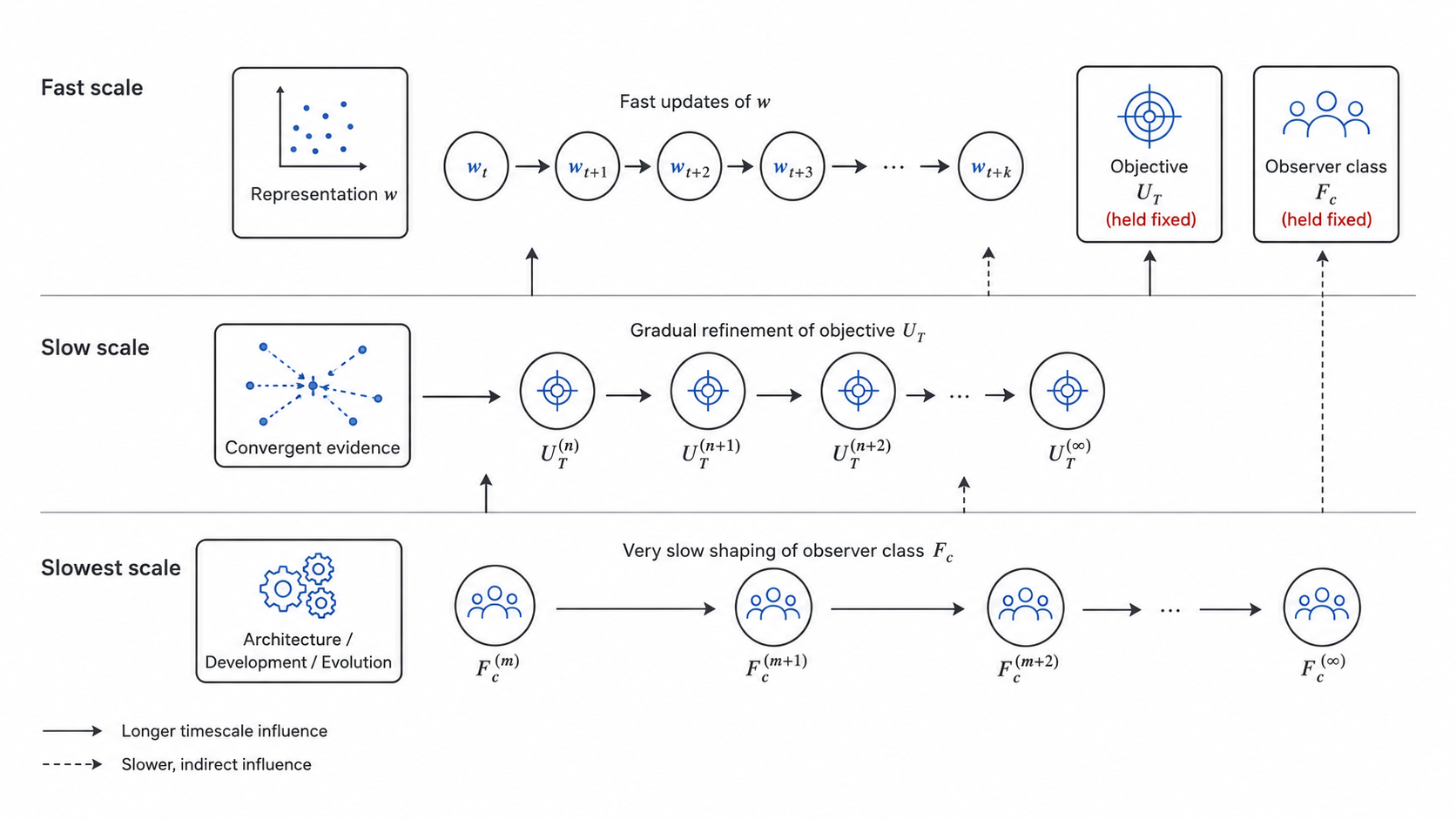
NLF makes the multiple timescales explicit. The fast scale is the one current ML mostly inhabits: given an objective $U_T$ and an observer class $\mathcal{F}$, find $w \in \mathcal{F}$ that approaches $w^{\ast}_T$. The slow scale governs the objective itself: how $U_T$ evolves under cross-task pressure, mechanistic constraints, and the convergent-evidence criteria of 2.3. The slowest scale governs the observer class: how $\mathcal{F}$ is shaped by architectural search, pretraining, curriculum, or, in biological systems, by development and evolution.
These three scales are not optional features of the framework. They are the only place where some of the most consequential phenomena in modern learning systems can be described at all. Pretraining and fine-tuning are not a single optimization but the interaction of two scales. Foundation models are not just large models; they are systems in which the slow-scale shaping of $U_T$ has been industrialized. The puzzles in 1, read in this light, are not three isolated phenomena but three different cross-sections of a single multi-scale process: an infant whose observer class has been shaped over evolutionary time, radiologists whose objectives have been shaped over career time, a softmax whose ideal is fixed at the fast scale by the geometry the slower scales have already established.
Closing the section
These five commitments, a task-grounded ideal, an explicit observer class, convergent justification, a structured residual, and explicit multiple timescales, are the working content of the Normative Learning Framework. They are not five independent ideas but five facets of a single structural claim: that learning is the approach of a bounded actor toward a target the data alone cannot specify, justified by evidence the actor cannot see directly, falling short in ways that themselves carry information, over timescales the immediate optimization does not name. The next section gives this structure its precise mathematical statement.
3 · The Normative Learning Framework: A Unified Definition
The previous section developed five commitments through which a learning system relates to a target the data alone does not specify. This section gives those commitments their precise mathematical statement. The five concepts of 2 become a structured set of objects, three coupled dynamics, and an analytical residual. The formalism that follows is intentionally compact. It is not a complete theory of learning. It is a vocabulary in which the puzzles of 1 and the commitments of 2 can be expressed without ambiguity, so that what comes next, the case studies of 4 and the future directions of 5, can be grounded in something more than analogy.
A note on convention. Throughout this section I use $U_T$ for the task-grounded objective, written as a quantity to be maximized. Readers more familiar with the loss formulation will recognize $U_T$ as the negative of a loss, with sign chosen to emphasize that the system is approaching a target rather than retreating from a penalty. The two formulations are equivalent, and I move freely between them when convenient.
3.1 · Objects
A Normative Learning problem is specified by the following.
A task environment $\mathcal{E}$ induces a (possibly time-varying) input distribution $P_t(x)$. The environment encompasses the physical world the system perceives, the social context it operates in, and the distribution of tasks it faces. It is what determines whether a given representation or behavior is adaptive at all.
An observer class $\mathcal{F}_c$ is the set of representations or policies a system can in principle realize. The subscript $c$ marks the dependence on a resource budget: compute, memory, training time, parameter count, and the plasticity budget $\Delta_t$, which bounds how much the parameters can change in unit time. In artificial systems, $c$ encompasses architectural scale, optimizer step size, distillation budgets, pruning ratios, and the numerical precision of computation. In biological systems, $c$ encompasses cortical area, metabolic supply, and synaptic plasticity bounds. The role of $c$ is the same in both: it determines what is reachable.
A task-grounded objective $U_T : \mathcal{F}_c \to \mathbb{R}$ is the formal object whose maximizer over $\mathcal{F}_c$ defines the normative ideal. It is the mathematical content of “what the system should approach.”
A meta-objective $\mathcal{M}(\mathcal{E})$ is the higher-order criterion under which $U_T$ itself is evaluated. $\mathcal{M}$ is rarely directly available, but its operational form, the convergent-evidence regularizer $\mathcal{R}$, is. $\mathcal{R}$ is the working approximation of $\mathcal{M}$ in any concrete analysis.
The output of a Normative Learning analysis is a normative ideal $w^{\ast}_T \in \mathcal{F}_c$ when the target is a representation, or $\pi^{\ast}_T \in \mathcal{F}_c$ when the target is a policy, together with a structured residual $\delta(w, w^{\ast}_T)$ describing how a realized system $w$ deviates from it.
These eight objects, $\mathcal{E}$, $P_t(x)$, $\mathcal{F}_c$, $U_T$, $\mathcal{M}$, $\mathcal{R}$, $w^{\ast}_T / \pi^{\ast}_T$, $\delta$, are the working vocabulary of the framework. Most existing analyses of learning systems can be recovered as specializations in which one or more of them is held fixed or implicit.
3.2 · Three coupled dynamics
The framework’s central structural claim is that a complete description of a learning system requires three nested timescales, each with its own dynamics.
The fast scale: representation learning under fixed objective.
Given $(U_T, \mathcal{F}_c)$, the system adapts its representation toward the ideal:
$$w^{\ast}_T \;\in\; \arg\max_{w \in \mathcal{F}_c} \; U_T(w), \quad \text{s.t.} \quad w \in \mathcal{M}(p(x)).$$
This is the scale at which most of contemporary machine learning operates. A loss is fixed, an architecture is fixed, a budget is fixed, and gradient descent, or its biological analogues, drives $w$ toward $w^{\ast}_T$. The plasticity budget $\Delta_t$ enters as a constraint on the per-step change in $w$, ensuring that adaptation is bounded by the resources available.
The slow scale: objective learning under convergent evidence.
The objective itself is not given; it is constrained by independent evidence and updated accordingly. The dynamics are
$$U_{t+1} \;=\; U_t \;-\; \eta_U \,\nabla_U\, \mathcal{R}(U_t; \mathcal{E}),$$
where $\mathcal{R}$ decomposes into the three terms described in 2.3:
$$\mathcal{R}(U_t; \mathcal{E}) \;=\; \alpha_1 \mathcal{R}_{\text{task}}(U_t; T) \;+\; \alpha_2 \mathcal{R}_{\text{cross}}(U_t; \{T_i\}) \;+\; \alpha_3 \mathcal{R}_{\text{mech}}(U_t; \text{obs}).$$
The first term penalizes objectives that cannot be derived from the formal structure of the task. The second penalizes objectives that fail to remain reasonable across related tasks. The third penalizes objectives whose predicted representations or behaviors conflict with independent observations. The mixing weights $\alpha_i$ are themselves determined, in principle, by the meta-objective $\mathcal{M}$, which is to say, by which kinds of evidence the broader environment treats as authoritative.
This is the scale at which pretraining, curriculum design, and the gradual refinement of learning objectives across years of research take place. It is the scale at which a community decides what its systems should be approaching, even if no individual researcher experiences the decision in those terms.
The slowest scale: observer-class shaping.
The observer class $\mathcal{F}_c$ is not given either. Architectures are searched, scaled, pruned, and selected; biological observers are shaped by development and evolution. At this scale, the relevant variables are the structural parameters that define $\mathcal{F}_c$ itself: depth, width, connectivity patterns, locality biases, plasticity profiles. Their evolution is governed by the same meta-objective $\mathcal{M}$ that shapes $U_T$, but with a different operational form: at this scale, what is being optimized is which class of $U_T$-and-$w$ pairs the system is even capable of representing.
I deliberately do not commit to a single formal expression for the slowest-scale update. Its operational form is domain-specific, ranging from neural architecture search and pretraining procedures in ML to development and evolution in biology, and forcing these into a common equation would purchase apparent generality at the cost of substantive content. The framework specifies that this update is governed by $\mathcal{M}$ and inherits the same convergent-evidence logic as the slow scale; it leaves the concrete form of “modify $\mathcal{F}_c$” to the system being analyzed.
Why three, and why these speeds.
The three scales are not chosen by inspection. They follow from a structural feature of the problem itself. The objects modified at each scale, $w$, $U_T$, and $\mathcal{F}_c$, are nested: each requires the previous to remain stable for its modification to be meaningful. Updating $w$ presupposes a fixed $U_T$, because gradient information becomes incoherent if the objective shifts during the update. Updating $U_T$ presupposes a fixed $\mathcal{F}_c$, because the convergent-evidence criteria of 2.3 cannot be evaluated until $w$ has converged across multiple datasets within $\mathcal{F}_c$. Updating $\mathcal{F}_c$ presupposes stability of $U_T$ across tasks, because architectural choices that improve some objective at the cost of others are not recognizable until the others have themselves been worked out.
This nesting fixes the speeds. The cost of modifying $w$ is one optimization step; the cost of modifying $U_T$ is one full learning run; the cost of modifying $\mathcal{F}_c$ is many learning runs across tasks. The three orders of magnitude in cost translate, by the same logic, into three orders of magnitude in the rate at which each object can be revised. This is not a stylized choice. It is the consequence of treating each layer’s effective sample size as the number of converged outcomes from the layer below: a single weight update gives one sample of $w$; a converged training run gives one sample of $U_T$’s adequacy; only an ensemble of training runs gives one sample of $\mathcal{F}_c$’s adequacy. Outer scales are slow because their evidence is, by construction, scarce.
The three-scale structure is therefore not an analytical convenience. It is the minimal decomposition under which each commitment in 2 has a well-defined operational meaning. Two scales would collapse $U_T$ and $\mathcal{F}_c$ into a single object and lose the distinction between objective shaping and architectural shaping. Four would split one of the three layers into substructures whose dynamics, on this analysis, are not separable. Three is what the structure of the problem allows.
The coupling.
The three scales are not independent. Each is the boundary condition of the next: the fast scale runs under a fixed $(U_T, \mathcal{F}_c)$; the slow scale modifies $U_T$ within a fixed $\mathcal{F}_c$; the slowest scale modifies $\mathcal{F}_c$ itself. A system that can be analyzed only at the fast scale is one whose slower scales have been held constant by external choice. Most ML analyses are exactly this kind of analysis, and most of the time this is appropriate. But when the slower scales matter, when pretraining matters, when architecture matters, when the very framing of the task is what is being learned, only the multi-scale structure can describe what is happening.
3.3 · The residual as analytical object
The framework’s central diagnostic tool is the structured residual:
$$\delta(w, w^{\ast}_T) \;=\; \delta^{\text{arch}} \;+\; \delta^{\text{train}} \;+\; \delta^{\text{approx}} \;+\; \delta^{\text{robust}} \;+\; \delta^{\text{multi}}.$$
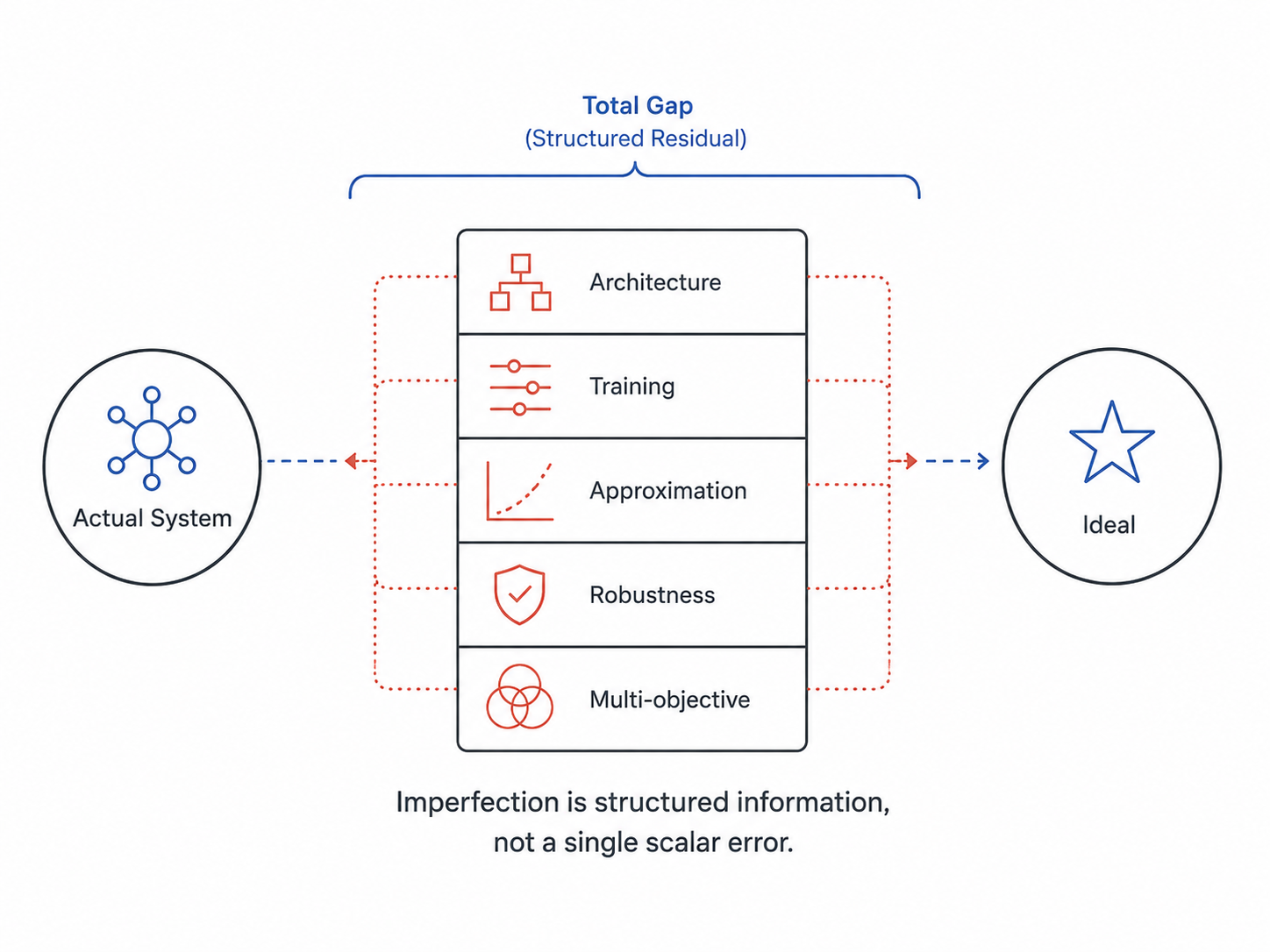
Each term corresponds to a distinct mechanism of departure from the ideal. $\delta^{\text{arch}}$ is the contribution of architectural and inductive-bias constraints, the gap between $w^{\ast}_T$ over the unbounded function space and the best element of $\mathcal{F}_c$. $\delta^{\text{train}}$ is the contribution of finite-sample, finite-step training, the gap between the best reachable in $\mathcal{F}_c$ and the actual $w$ produced by the learning process. $\delta^{\text{approx}}$ is the contribution of approximation in the objective itself, the gap between the realized $U_T$ and the more accurate normative target it surrogates. $\delta^{\text{robust}}$ is the contribution of deliberate margins held against distribution shift or rare events. $\delta^{\text{multi}}$ is the contribution of competing objectives the system is balancing simultaneously.
Each term has distinct empirical signatures and distinct interventions. Architectural residual is reduced by changing $\mathcal{F}_c$; training residual is reduced by changing the optimization procedure; approximation residual is reduced by sharpening $U_T$; robustness residual cannot be reduced without losing the protection it provides; multi-objective residual cannot be reduced without abandoning one of the objectives. To collapse all of them into a single accuracy gap is to make every one of these distinctions invisible.
The residual is not a measure of failure. It is the analytical object that turns “is the system optimal?” into “where, and why, and at what cost, does this system fall short of what it should be approaching?” The answer to the second question is the scientific content the first question discards.
3.4 · Lineage
The Normative Learning Framework synthesizes commitments from several traditions that have, in different communities and different vocabularies, insisted on essentially the same idea: that representations and behaviors of intelligent systems should be evaluated against task-derived ideals rather than convenience-chosen losses.
Efficient coding (Barlow, 1961; Atick, 1992) and its modern Bayesian extensions (Park & Pillow, 2017; Młynarski & Hermundstad, 2018) developed the original commitment for sensory systems: representations should maximize task-relevant information under capacity constraints. Ideal observer analysis (Geisler, 2003; Burgess, 1981) developed it for perception: observed performance should be measured against the optimal extractor of task-relevant information from the available signal. Rational analysis (Anderson, 1990) and its resource-rational refinement (Lieder & Griffiths, 2020) developed it for cognition: behavior should be understood as optimal under explicit resource bounds. Active inference (Friston, 2010) developed it for sensorimotor systems: actions are selected to minimize expected free energy. Causal representation learning (Schölkopf et al., 2021) developed it for representation: the right ideal is one that recovers the causal structure of the data-generating process.
What I claim as contribution is not any one of these ingredients. It is the articulation of their joint necessity, the explicit multi-scale structure that distinguishes objective from architecture from optimization, and the residual-as-signal methodology that the case studies of 4 will demonstrate. NLF is built on the premise that these traditions have been describing facets of the same object, and that progress in each is bounded by the limits of describing it from one side at a time.
4 · The Framework at Work: Research Program
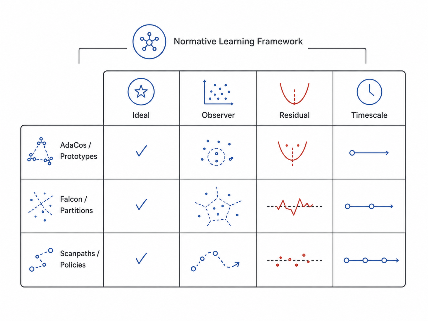
The framework of 3 was developed in dialogue with three lines of my own research, and three more open questions it has helped me see. This section presents the research lines themselves, organized not as a chronological account of the papers but as concrete instantiations of the framework: each illustrates how a particular NLF object, task-grounded ideal, observer class, residual structure, does scientific work when taken seriously. The lines span representation and behavior, supervised and unsupervised regimes, static $w^{\ast}_T$ and sequential $\pi^{\ast}_T$. Together they map the framework’s working surface.
4.1 · Prototypes: task-theoretic ideals in deep recognition
This line instantiates the task-grounded objective $U_T$ (2.1) in the supervised regime, illustrating the methodological shift from tuning hyperparameters to deriving them from task structure.
The task and the ideal.
Deep metric learning, of which face recognition is the canonical instance, asks for embeddings under which same-identity samples cluster tightly and different-identity samples separate. The dominant approach has been a decade of empirical loss engineering: SphereFace, CosFace, ArcFace, and a long tail of margin-based softmax variants, each introducing additional hyperparameters tuned by ablation. The community treated the scale factor $s$ and the margin $m$ as free design choices.
NLF reframes the question. Under a probabilistic model of embeddings on the unit hypersphere, the von Mises-Fisher distribution, the task-grounded ideal $w^{\ast}_c$ for each identity $c$ is the prototype that maximizes posterior discriminability given the embedding geometry. Crucially, $s$ and $m$ are not free: they are determined by the requirement that the surrogate softmax distribution be probabilistically calibrated against the underlying von Mises-Fisher posterior. The hyperparameters belong to $U_T$, not to engineering.
The methods.
AdaCos (CVPR 2019, Oral) made this derivation concrete. Under the calibration condition, the optimal scale at training step $t$ admits a closed form,
$$s_t \;=\; \frac{\log B_{\text{avg}}}{\cos \theta_{\text{med}}},$$
where $B_{\text{avg}}$ is the average exponentiated negative-class logit and $\theta_{\text{med}}$ is the median positive-class angle. The hyperparameter people had been tuning was a quantity already implicit in the gradient signal.
P2SGrad (CVPR 2019) extended the same normative move to the gradient level itself. The numerical magnitudes that scale and margin parameters introduce into gradient updates are surrogate artifacts; eliminating them yields an optimization signal that directly reflects angular discriminability without distortion.
RBF-Softmax (ECCV 2020) parameterized the prototype geometry explicitly through radial basis functions, making the convergence of $w_c$ trajectories interpretable as Gaussian-process-style ideal clustering with tractable likelihood.
Reading the residual.
Within NLF, these methods all target $\delta^{\text{approx}}$, the gap between the surrogate cosine-softmax loss and its probabilistically-calibrated form. After this gap is closed, what remains of the residual is informative rather than noisy: $\delta^{\text{train}}$ becomes a clean signal of finite-sample coverage limits, useful for curriculum design, and $\delta^{\text{robust}}$ becomes visible as a deliberate margin against identity-OOD conditions. Closing one component of the residual is what allows the others to be diagnosed.
What the case demonstrates.
This line illustrates the minimal form of normative methodology: from tuning a loss to deriving an objective. It demonstrates that even in a domain dominated by empirical loss engineering, the move from chosen hyperparameter to derived quantity is operationally tractable, and that the gain is not only better performance but a clearer scientific picture of what the system is doing.
4.2 · Partitions: data-geometric ideals in unsupervised structure
This line instantiates the data-geometric branch of $U_T$ (2.1) and the observer-class constraint $\mathcal{F}_c$ (2.2), demonstrating that normative ideals can be defined without any labels, drawn directly from the structure of data.
The task and the ideal.
When labels are absent, the question “what is the ideal?” cannot be deferred to supervision. It must be answered by data geometry itself. The canonical formulation is Normalized Cuts (Shi & Malik, 2000): the ideal partition $w^{\ast}$ is the one minimizing the normalized cut over a perceptual affinity graph, grounded in Gestalt grouping principles and, conjecturally, in the lateral connectivity patterns of early visual cortex. The ideal is well-defined, decades old, and theoretically clean. The scientific challenge has not been conceptual, it has been computational. Classical NCut scales as $O(n^3)$ in the number of nodes and has no straightforward extension to learned deep features.
The methods.
Falcon (ICLR 2026) resolves the scalability problem through proximal linearization. Rather than solving the relaxed NCut eigenproblem directly, the method linearizes the cut functional around the current iterate and adds a trust-region term:
$$w_{k+1} \;=\; \arg\min_w \Big\{ \langle \nabla f(w_k),\, w \rangle \;+\; \tfrac{1}{2\tau}\|w - w_k\|^2 \Big\},$$
where $f$ is the relaxed normalized cut over a deep feature affinity graph. The reformulation preserves the normative content of NCut, what is approached is unchanged, while making the approach itself tractable for the deep, large-scale feature spaces of modern vision systems. The scientific contribution is not a new objective. It is the scaling of an old normative formulation into a regime where it had been thought to be unreachable.
Clustering Consensus (CVPR 2021) addresses a complementary scenario, in unsupervised person re-identification, where neither labels nor a fixed affinity graph is available. I formalized the unsupervised prototype as the fixed point of an iterative self-consistency map:
$$w^{(t+1)} \;=\; \mathbb{E}_x\big[\phi(x) \,\big|\, q(y \mid x; w^{(t)})\big],$$
with identifiability established through cross-generation agreement. The normative ideal here is not specified in advance; it emerges as the convergence point of the system’s own consistency dynamics.
Reading the residual.
Falcon’s residual is dominated by $\delta^{\text{approx}}$ against the spectral ideal, and the surviving residual reflects $\delta^{\text{multi}}$, the intrinsic multi-scale ambiguity of natural images. This is information, not failure: a single partition is a Pareto compromise across resolutions the data itself supports. Clustering Consensus instead addresses $\delta^{\text{arch}}$, in the sense that the absence of an external affinity graph is itself a structural constraint, partially resolved by constructing the affinity from the system’s own representation dynamics.
What the case demonstrates.
This line shows that the normative ideal can live entirely in data geometry, requiring no labels and no external supervision. It also shows that “scaling a classical normative formulation” is itself a substantive methodological move, not all progress in normative learning requires inventing new objectives; some of it is making old ideals reachable.
4.3 · Scanpaths: sensorimotor ideals in expert perception
This line extends NLF from static representations $w^{\ast}_T$ to sequential policies $\pi^{\ast}_T$, and is the most complete current instantiation of the residual-as-signal methodology (2.4) and the multi-scale structure (2.5).
The task and the ideal.
Radiologists reading chest X-rays and CT scans face a sensorimotor problem: each fixation is an action that reshapes the next observation, and the goal is reliable lesion detection under perceptual, temporal, and cognitive constraints. The normative ideal is no longer a single representation but a policy, $\pi^{\ast}_T$, the fixation sequence that maximizes expected diagnostic information under the observer’s perceptual architecture. Ideal observer analysis (Geisler, 2003) provides the theoretical form of $\pi^{\ast}_T$. What it has historically lacked is a scalable computational path from theoretical $\pi^{\ast}_T$ to measured clinician behavior, and a vocabulary for describing how individual clinicians fall short of it.
The methods.
The ongoing project comprises three interlocking technical components, each a substantive research thrust in its own right.
First, controllable conditional generative models for CXR and CT, conditioned on structured clinical variables: pathology type, anatomical region, presentation difficulty, demographic factors. These models enable perceptual experiments at scale, with each visual stimulus dimension manipulable independently of the others. Without controllable stimuli, $\pi^{\ast}_T$ can be theoretically defined but not empirically probed across a sufficient range of conditions.
Second, scanpath generation models that parameterize candidate fixation policies $\pi_\theta$. Trained on expert demonstrations under structured inverse reinforcement learning, these models produce policy distributions whose distance to $\pi^{\ast}_T$, under appropriately defined metrics over fixation sequences, becomes computable. This converts the theoretical ideal into a concrete reference object.
Third, mechanistic decomposition of expertise. A clinician’s deviation from $\pi^{\ast}_T$ is not collapsed into a single skill score. It is parsed along interpretable axes: texture-based salience sensitivity, spatial efficiency of search, temporal dwell allocation on diagnostic regions, robustness margins on rare pathologies. The output is not a number but a profile.
Reading the residual.
This is where the residual decomposition of 2.4 becomes the scientific instrument, not a post-hoc analysis layer. A junior radiologist’s gap to $\pi^{\ast}_T$ decomposes into $\delta^{\text{train}}$ (limited case exposure during training), $\delta^{\text{approx}}$ (heuristic search rather than optimal information-theoretic planning), and $\delta^{\text{robust}}$ (deliberate over-fixation margins on rare pathologies, sometimes adaptive and sometimes not). Each component points to a distinct training intervention, distinct from the others in both mechanism and remedy. Expertise assessment, which clinical practice has historically reduced to coarse experience-based metrics, becomes a diagnostic profile with direct implications for radiologic education and certification.
What the case demonstrates.
This line realizes the framework’s full methodology in a single project: the ideal is normatively specified, approached scalably, and its residual read as the primary scientific object, with measurable consequences for medical training and clinical practice. It demonstrates that NLF’s methodology transfers from representation to behavior without conceptual modification, and that the move from $w^{\ast}$ to $\pi^{\ast}$ opens new applied territory the static framework alone cannot reach.
Closing the section
Across representation and behavior, static $w^{\ast}_T$ and sequential $\pi^{\ast}_T$, supervised and unsupervised settings, these three lines share a single architecture: identify the normative ideal, build scalable mechanisms that approach it, and treat the residual as the primary object of analysis. Each case populates a different cell of the framework. AdaCos and its successors instantiate the task-theoretic source of $U_T$ in a supervised regime. Falcon and Clustering Consensus instantiate the data-geometric source of $U_T$ without labels. The radiology project extends the entire framework to sensorimotor policies, with the residual as the working scientific output.
What unifies them is not a method or a domain. It is a methodological commitment: that the right starting point in any learning problem is the question of what the system should be approaching, and that the right scientific output is not whether it succeeds but how, where, and at what cost it falls short.
5 · Future Directions
The Normative Learning Framework, as I have presented it, is deliberately incomplete. Each of its commitments opens a research program rather than closing one. Three directions occupy the largest part of my work over the coming years. They are not arbitrary choices: each extends the framework along an axis that current work touches but has not yet formalized, and each corresponds to an underdeveloped element of NLF that the case studies of 4 have begun, but not finished, to populate.
Direction 1 · Multimodal and Causal Normative Ideals
The framework as I have stated it treats $U_T$ as scalar and the input distribution $P_t(x)$ as effectively unimodal. Modern learning systems do not. Vision-language models, embodied agents, and multimodal foundation systems all operate over heterogeneous input streams in which the right ideal depends on which modalities are integrated, in what order, and under what causal structure. The literature on these systems has grown rapidly, but it lacks a principled way to ask what their normative target should be, as distinct from what their training loss happens to be.
I plan to formalize multimodal $U_T$ in two complementary ways. The first is structural: $U_T$ should depend on the causal direction of dependencies among modalities, not merely their statistical correlations. Building on causal representation learning (Schölkopf et al., 2021), I aim to write down identifiability conditions under which a multimodal $U_T$ separates genuine cross-modal grounding from shortcut exploitation of language leakage in vision tasks, of dataset artifacts in cross-modal alignment, of spurious co-occurrence in embodied training. The second is diagnostic: applying the residual decomposition of 2.4 to deployed multimodal systems, treating the structural difference between $\delta^{\text{approx}}$ (the model approximates the wrong $U_T$) and $\delta^{\text{arch}}$ (the model’s architecture cannot represent the right $U_T$) as the central scientific question. This direction extends 4.1 and 4.2 from single-modality representation to multimodal, causally grounded representation, and treats shortcut learning not as a failure mode to patch but as a residual signal to read.
Direction 2 · Sensorimotor Normative Learning as a Scientific Program
The radiology project of 4.3 is one instance of a broader claim. NLF applied to sensorimotor policies, to $\pi^{\ast}_T$ rather than $w^{\ast}_T$, has the potential to provide a common mathematical language across domains where expertise has resisted quantification. Surgery, flight, instrument performance, second-language acquisition, and educational assessment all share a structural feature: an observable sensorimotor policy, a normatively definable ideal, and learners whose distance to the ideal carries practical and theoretical content.
My program here has two arms. The first is methodological: I aim to develop the Ideal-Observer Policy Benchmark, a multi-domain testbed for measuring $d(\pi_{\text{human}}, \pi^{\ast}_T)$ with mechanistic decomposition along interpretable axes. The second is applied: pursuing clinical deployment of the radiology pipeline as a concrete instance of operational expertise assessment, in collaboration with medical institutions, with the goal of replacing coarse experience-based metrics with mechanism-based diagnostic profiles. The broader scientific claim under test is that NLF’s residual-as-signal methodology transfers cleanly from representation to action, giving cognitive science and the applied sciences a shared vocabulary for describing skill, where it comes from, and how it falls short.
Direction 3 · Residual Diagnostics as a Methodological Discipline
The residual decomposition of 2.4 is, at present, a methodological commitment I apply by hand to my own work. The case studies of 4 illustrate what it can do; they do not yet demonstrate that anyone else can do it. The third direction of my research is to make the residual analysis a tool others can use, on systems they care about, without reproducing the case-by-case derivations that currently make it work.
Concretely, I aim to develop normative attribution methods: computational procedures that, given a trained model and a specified normative ideal, automatically decompose the model’s deviation from that ideal along the components $\delta^{\text{arch}}, \delta^{\text{train}}, \delta^{\text{approx}}, \delta^{\text{robust}}, \delta^{\text{multi}}$. Applied to current foundation models, such tools would distinguish whether a vision-language model’s failure on a particular reasoning task reflects an architectural bottleneck, a training-data gap, an objective misalignment, or a robustness margin the system is correctly preserving. Each diagnosis points to a different fix. The longer-term ambition is for normative debugging to become a standard stage of model development, alongside accuracy benchmarking and ablation, providing a structured account of where systems fall short and why.
This direction treats the framework’s analytical signature as a discipline in its own right. It is the move from “I find this useful” to “this is how the field should think.” Whether the move succeeds is an empirical question, to be answered by whether other researchers find the tools worth picking up. I take that question seriously, and the next phase of the work is designed around it.
Closing
The three puzzles that opened this statement have a common shape: in each, a learning system is approaching something the data alone does not specify. The five commitments of 2 named the structure of that approach. The formalism of 3 gave it precise mathematical content. The case studies of 4 showed the framework doing work in concrete research, and the directions of 5 show where I believe the work is going.
What I am proposing is not a theory of learning. It is a vocabulary in which the question of what learning is for can be asked precisely, answered with structure rather than with a single number, and shared across the disciplines that currently describe pieces of the same object from incompatible angles. The work ahead is to keep articulating that vocabulary, to extend it where the puzzles demand, and to build the tools that turn it from a personal research program into a shared methodology. That is what I take my research, and the years of it that follow, to be about.